Summer Fun

Every Spring I have a lot of fun proofreading Audrey Weeks’ new Calculus in Motion illustrations for the most recent AP Calculus Exam questions. These illustrations run on Geometers’ Sketchpad. In addition to the exam questions Calculus in Motion (and its companion Algebra in Motion) include separate animations illustrating most of the concepts in calculus and algebra. This is a great resource for your classes.

The proofreading and the cross-country conversations with Audrey give me a chance to learn more about the questions.

This year, I really got into 2018 AB 6, the differential equation question. I wrote an exploration (or as the kids would say “worksheet”) on a function very similar to the differential equation in that question. The exploration, which is rather long, includes these topics:

  • Finding the general solution of the differential equation by separating the variables
  • Checking the solution by substitution
  • Using a graphing utility to explore the solutions for all values of the constant of integration, C
  • Finding the solutions’ horizontal and vertical asymptotes
  • Finding several particular solutions
  • Finding the domains of the particular solutions
  • Finding the extreme value of all solutions in terms of C
  • Finding the second derivative (implicit differentiation)
  • Considering concavity
  • Investigating a special case or two

I also hope that in working through this exploration students will learn not so much about this particular function, but how to use the tools of algebra, calculus, and technology to fully investigate any function and to find all its foibles.

Students will need to have studied calculus through differential equations before they start the exploration. I will repost it next January for them.

The exploration is here for you to try. Try it before you look at the solutions. It will give you something to do over the summer – well not all summer, only an hour or so.

As always, I appreciate your feedback and comments. Please share them with me using the reply box below.


There will be only occasional, very occasional, posts over the Summer. More regular posting will begin again in August. Enjoy the Explorations, and, more important, enjoy the Summer!

.


Getting Ready

Today we continue to look at some previous posts that I hope will help you and your students throughout the year. We begin with some posts on graphing calculator use and then a few general things in three posts on beginning the year, followed by some mathematics I hope students know before they start studying the calculus.

Graphing Calculators

There are four things that students may, and are required to know how to do, for the AP Exams. But graphing calculators are not required just to answer a few questions on the exams. They are to encourage investigations and experimentation in all math classes. And not just graphing calculator use but all kinds of appropriate technology. So, don’t restrict yourself and your students to only those operations required on the exam. That said, here are previous posts on exam calculator use; as the year goes on there will be other posts on the use of graphing calculators and other technology in your class.

Starting School

A little late perhaps …

These posts discuss basic ideas that I always hoped students knew about mathematics before starting calculus


.

Graphing Integrals

The sixth in the Graphing Calculator / Technology series

The topic of integration is coming up soon. Here are some notes and ideas about the integration operation on graphing calculators. The entries are the same or very similar for all calculator brands.

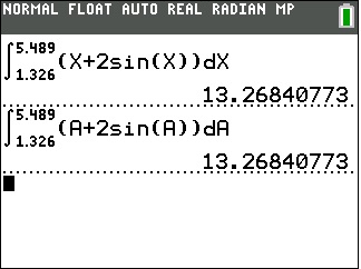
The basic problem of evaluating a definite integral on a graphing calculator is done without finding an antiderivative; that is, the calculator uses a numerical algorithm to produce the result. The calculator provides a template,integral-templateand you fill in the 4 squares so that the expression looks exactly like what you write by hand. Then the calculator computes the result. (Older models require a one-line input requiring, in order, the integrand, the independent variable, the lower limit of integration and the upper limit in that order, separated by commas.) The first interesting thing is that the variable in the integrand does to have to be x. As the first figure illustrates using x or a or any other letter gives the same result.

integral-0

This is because the variable of integration is just a place holder. Sometimes called a “dummy variable”, this letter can be anything at all, including x. On the home or calculation screen you might as well always use x, so the entry will look like what you have on your paper. As we will see, when graphing it may be less confusing to use a different letter.

The antiderivative, F, of any function, f, can be written as a function defined by an integral where there is a point on the antiderivative of f , which is with F ’ = f. The point (aF(a)) is the initial condition. (In the following we will use F(a) = 0 as the initial condition – the graph will contain the origin. As a further investigation, try changing the lower limit to different numbers and see how that changes the graph.)

The integration operation can be used to graph the antiderivative of a function without finding the antiderivative. You may graph the antiderivative when teaching antiderivatives. Have students look at the graph of the antiderivative and guess what that function is.

When graphing use x as the upper limit of integration and a different letter for the variable in the rest of the template. The calculator will use different values of x to calculate the points to be graphed.

The set-up shown in the next figure shows how to enter a function defined by an integral (blue line) and the same function obtained by antidifferentiating (red squares). As you can see the results are the same.

integral-1

In this way, you can explore the functions and their indefinite integrals by graphing.

The Fundamental Theorem of Calculus

Another use of using the graph of an integral is to investigate both parts of the Fundamental Theorem of Calculus (FTC). Roughly speaking, the FTC says that the integral of a derivative of a function is that function, and the derivative of an integral is the integrand.

In the figure below, the same function is entered both ways; the graphs are the same. (Note the x’s in the second line must be x in all four places.)

integral-2

.

How to Tell your Asymptote from a Hole in the Graph.

The fifth in the Graphing Calculator / Technology series

(The MPAC discussion will continue next week)

Seeing discontinuities on a graphing calculator is possible; but you need to know how a calculator graphs to do it. Here’s the story:

The number you choose for XMIN becomes the x-coordinate of the (center of) the pixels in the left most column of pixels. The number you choose for XMAX is the x-coordinate of the right most column of pixels. The distance between XMIN and XMAX is divided evenly between the remaining pixels so that all the pixels are evenly spaced across the screen (the same distance apart). The rows of pixels are done the same way evenly spacing them between YMIN and YMAX.

This spacing is usually not at “nice” values as can be seen by just moving the cursor across the screen and noticing the x-values or y-values at the bottom of the screen.

The cursor is located one pixel to the right of the y-axis and one pixel above the x-axis in the “standard” window of a TI-8x. Note the coordinates of that pixel at the bottom of the screen.

The cursor is located one pixel to the right of the y-axis and one pixel above the x-axis in the “standard” window of a TI-8x. Note the coordinates of that pixel at the bottom of the screen. These are the distances between the pixels.

To draw a graph, the calculator takes the x-coordinate of each pixel, calculates the corresponding y-value and turns on the pixel in that column with closest y-pixel-coordinate. If set in a connect mode, the calculator turns on several pixels in adjacent columns so that the y-values seem to connect; this is why the graph often looks jagged in steep sections of the graph. If you are in DOT mode, this does not happen and only one pixel in each column is on.

If you move the cursor over one of the points on a graph, you will see the pixel coordinates, NOT the actual y-coordinates. Use TRACE to see the actual y-coordinate. This is why when finding intersections, you should not just move the cursor over the point, but rather use “intersect” to see the actual y-value of the function.

If the function is undefined for some x-pixel value, then no pixel will turn on in that column. If the function is undefined for some value between the pixel values, then nothing happens because the calculator has not evaluated the function there, so the graph seems to be continuous.

Vertical “asymptotes” are the result of the calculator not evaluating the function at the undefined value; rather it connects the value on one side of the asymptote off the bottom of the screen with the next value on the other side of the asymptote off the top of the screen. If the asymptote appears exactly at a pixel value, then no “asymptote” will appear and that column of pixels will have no pixel turned on. (Some newer calculators and newer operating systems on older calculators have made adjustments so that the “asymptotes” do not show up. In some systems this feature can be turned on or off.)

The function $latex \displaystyle y=\frac{3\left( x-2 \right)}{\left( x-2 \right)\left( x+2 \right)}$ in the standard window. The vertical line is not really the asymptote and the “hole” at (2, 0.75) is not seen.

The function \displaystyle y=\frac{3\left( x-2 \right)}{\left( x-2 \right)\left( x+2 \right)} in the standard window. The vertical line is not really the asymptote and the “hole” at (2, 0.75) is not seen.

A removable discontinuity, a hole in the graph (really a skipped pixel), can be seen, if it occurs at a pixel value. Since in most examples the hole is at an integer or other “nice” number, you will not see them in the “standard” window. Use a “decimal” window, which has been chosen in advance so the x-values of the pixels are integers and nice decimals. (To see this, in a decimal window move the cursor around and notice the pixel coordinates).

The other thing you can do is adjust the XMIN and XMAX values so that the distance between them will land on integer values. (Nice project for your class – the number of pixels can be found in the guidebook, or you can count them. In the old days, before decimal windows, this was necessary – it was called finding a “friendly window.”)

The function $latex \displaystyle y=\frac{3\left( x-2 \right)}{\left( x-2 \right)\left( x+2 \right)}$ in the “decimal” window. The “asymptote” is not shown and the “hole” at (2, 0.75) is visible.

The function \displaystyle y=\frac{3\left( x-2 \right)}{\left( x-2 \right)\left( x+2 \right)} in the “decimal” window. The “asymptote” has disappeared and the “hole” at (2, 0.75) is now visible.

Zooming in or out may change these values so the hole or asymptote disappears.

For a related idea see the post My Favorite Function


PLEASE NOTE: I have no control over the advertising that appears on this blog. It is provided by WordPress and I would have to pay a great deal to not have advertising. I do not endorse anything advertised here. I noticed that ads for one of the presidential candidates occasionally appears; I certainly do not endorse him.


Tangent Lines

Second in the Graphing Calculator/Technology series

This graphing calculator activity is a way to introduce the idea if the slope of the tangent line as the limit of the slope of a secant line. In it, students will write the equation of a secant line through two very close points. They will then compare their results in several ways.

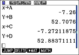
Begin by having the students graph a very simple curve such as y = x2 in the standard window of their calculator. Then TRACE to a point. Students will go to different points, some to the left and some to the right of the origin. ZOOM IN several times on this point until their graph appears linear (discuss local linearity here). To be sure they are on the graph push TRACE again. The coordinates of their point will be at the bottom of the screen; call this point (a, b). Return to the home screen and store the values to A and B (click here for instructions on storing and recalling numbers).

Return to the graph and push TRACE again to be sure the cursor is on the graph. Move the TRACE cursor one or two pixels away from the first point in either direction. This new point is (c, d). Return to the home screen and store the coordinates to C and D.

calc 2.1

Enter the equation of the line through the two points on the equation entry screen in terms of A, B, C, and D. Zoom Out several times until you have returned to the original window..

calc 2.4

Exploration 1: Have students compare and contrast their graphs with several other students and discuss their observations. (Expected observations: the lines appear tangent at each students’ original point)

Exploration 2: Ask student to compute the slope of the line through their points, again using A, B, C, and D. Collect each student’s x-coordinate, A, and their slope and enter them in list is your calculator so that they can be projected.

calc 2.2

Study the two lists and discuss the relation is any. (Expected observations: the slope is twice the x-coordinate.) Can you write an equation of these pairs? (Expected result: y = 2x)

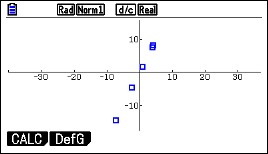
Finally, plot the points on the calculator using a square window. Do the points seem to lie on the line y =2x?

calc 2.3

Extensions:

Try the same activity with other functions such as y = (1/3)x3, y = x3, or y = x4. Anything more difficult will still result in a tangent line, but the numerical relationship between x and the slope will probably be too difficult to see. You may also consider y = sin(x) or y = cos(x). Again, the numerical work in Exploration 2, will be too difficult to see, but on graphing the points the result may be obvious. For y = sin(x), return to the list and add a column with the cosines of the x-values. Compare these with the slopes.

Graphing Calculator Use

First in a series. 

I am going to (try to) write a series of posts this fall on graphing calculator use in for calculus. Graphing calculators became generally available around 1989 and were made a requirement for use on the AP calculus exams in 1995. The hope was that they would encourage the use of technology generally in all math classes, and to an extent this has happened. In the coming posts I hope to show how graphing calculators can be used beyond the four skills required for the AP exams to help students understand what’s going on.

I will occasionally work with CAS calculators, but the main focus will be the basic non-CAS graphing calculators. All the suggestions will work of CAS calculators, of course. Also, I will occasionally make use of Desmos a free online graphing utility that students can easily access on their computer, tablet or smart phone.

Today I will discuss the four things students should be able to do, and in fact are required to do, on the AP exams. I will also show how to store and recall numbers. This last skill, while not required, is very useful. I have found that some teachers, and therefore their students, are unaware of this common feature of graphing calculators.

Calculators and other technology should be available from at least Algebra 1 on. So by the time students get to calculus calculator use (except for the calculus specific operations) should all be second nature to them.

So let’s get going. Here are the four required skills and some brief comments on each.

  1. Graph a function in a suitable window. The exam questions do not say “use a calculator”, so students are expected to know when seeing a graph will help them. The viewing window is not usually specified either so students should be familiar with setting the viewing window. If the domain is given in the question, then that’s what the students should use. If no domain is given, then use a range that includes the answer choices.
  2. Solve an equation numerically. Students may use any built-in feature to do this. The home screen “solver”, a routine called “Poly” or “Poly solve” are all allowed. Probably the most useful is to graph both sides of the equation and then use the graph operation called “intersect” to find the points of intersection one at a time. Another approach is to set the equation equal to 0, graph that expression and use the “roots” or “zeros” operations to solve the equation.
  3. Find the value of the derivative of a function at a given point. There is a built-in template for this.
  4. Find the value of a definite integral. There is a built-in template for this also.

Store-and-Recall

I will demonstrate the store-and-recall idea with an example that will also use skill 1, 2, and 4 from the list above.

Example: Find the area between the graph of f(x) = ln(x) and g(x) = x – 2, using (1) vertical rectangles, and (2) using horizontal rectangles.

For either method we need the coordinates of the points of intersection of the graphs. So, begin by graphing the functions and adjusting the window so the important points are visible.
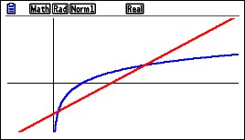
calc 1Next use the intersection operation to find the first point of intersection.
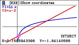
calc 2

Different calculators will do this slightly differently. The coordinates of the points of intersection are shown at the bottom of the screen. Think of this point as (a, b). The coordinates need to be stored for use later. To do this return to the home screen and type

[x] [STO], [alpha] [A]    and    [alpha] [y] [STO] [alpha] [B]

If your graph screen shows different names, such as xc and yc, then type that befroe the [STO] key. (The store [STO] key may look like an arrow pointing right.)
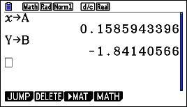
calc 3

Return to the graph screen and find the coordinates of the second point of intersection; think of this as (c, d). Return to the home screen and store the coordinates as C and D. They are c = 3.146193221 and d = 1.146193221.

To find the area use the definite integral template and enter the information needed. For the vertical rectangles you may use either the function or Y1 and Y2 that you entered to graph.
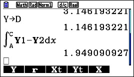
calc 4

Notice that the upper and lower limits of integration are A and C. The calculator uses the values you stored in these locations. You can use the variables in any kind of computation.

Here is the horizontal rectangle computation using B and D as limits. The functions solved for y are x = y + 2 on the right and x = ey on the left. (The y’s have been changed to x’s since the template only allows x as a variable.)
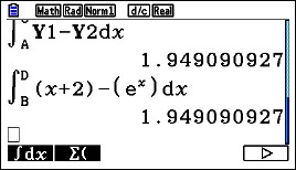
calc 5

Notice that so far, we’ve written nothing down. Everything has been done on the calculator. This prevents copy errors and round-off errors.

What should a student show on his or her AP Exam? They are required to show what they are doing, or more precisely what they’ve asked their calculator to do. They need to write the equation they are solving with the solution next to it, but no intermediate work. They should indicate what A and C are. So

\ln (x)=x+2,\ x=0.158594\text{ and }x=3.146193

a=0.158594\text{ and }c=3.146193

Then show the integral and answer. Here again they may use f and g given in the stem or the actual expressions. There is no requirement that answers must be given to three decimal places, so there is no need to round.

\displaystyle \int_{a}^{c}{f\left( x \right)-g\left( x \right)dx}=1.94909

The next post in this series will show you a way to introduce the idea odf the derivative as the slope of the tangent line.

Good Question 8 – or not?

Seattle rainToday’s question is not a good question. It’s a bad question.

But sometimes a bad question can become a good one.

This one leads first to a discussion of units, then to all sorts of calculus.

Here’s the question a teacher sent me this week taken from his textbook:

The normal monthly rainfall at the Seattle-Tacoma airport can be approximated by the model R=3.121+2.399\sin \left( 0.524t+1.377 \right), where R is measured in inches and t is the time in months, t = 1 being January. Use integration to approximate the normal annual rainfall.  Hint: Integrate over the interval [0,12].

Of course, with the hint it’s not difficult to know what to do and that makes it less than a good question right there. The answer is \displaystyle \int_{0}^{12}{R(t)dt=37.4736} inches. You could quit here and go on to the next question, but …

Then a student asked. “If R is in inches shouldn’t be in units of the integral be inch-months, since the unit of an integral is the unit of the integrand times the units of the independent variable?”  Well, yes, they should. So, what’s up with that?

Also, the teacher figured that the integral of a rate is an amount and our answer is an amount, so why isn’t the integrand a rate?

The only answer I could come up with is that the statement “R is measured in inches” is incorrect; R should be measured in inches /month. The opening phrase “normal monthly rainfall” also seems to point to the correct units for R being inches/month.

Problem solved; or maybe does this lead to a different concern?

The teacher pointed out that R(6) = 0.7658 inches is a reasonable answer for the amount of rain in June whereas \displaystyle \int_{0}^{6}{R(t)dt=}20.4786 is not.

If R is a rate, then the amount of rain that falls in June (t = 6) is given by \displaystyle \int_{5}^{6}{R(t)dt}=0.9890.

From here on we will assume that R is a rate with units of inches/month. Here are the individual monthly rates calculated with a CAS. Ques 8 a

The total amount of rainfall (second line above) appears be R(1) + R(2) + R(3) + … +R(12) = 37.4742. This is very close to the amount calculated by integration.

The slight difference of 0.0006 is not a round off error.

Remember, behind every definite integral there is a Riemann sum!

Again, the units are the problem. Why does the sum of the monthly rates seem to give the total amount?  The reason is that the terms of the sequence above are actually the values of a right-side Riemann sum of the rate, R(t), over the interval [0,12] with 12 equal subdivisions of width 1 (month) each with the 1’s left out as 1’s often are. Therefore, their sum should come close to the total yearly rainfall, but it is really just an approximation of it.

The actual total for any month, n, is given by \displaystyle \int_{n-1}^{n}{r(t)}dt. For example the amount of rain that falls in June is given by \displaystyle \int_{5}^{6}{R(t)dt}=0.9890 inches.

Here is the sequence of the actual monthly rainfall values in inches, and their sum.

Ques 8 b

This agrees with the integral. Why? Because one of  the properties of integrals tell us that \displaystyle \sum\limits_{n=1}^{12}{\int_{n-1}^{n}{r(t)dt}}=\int_{0}^{12}{r(t)dt}.


Another instructive thing with this integral is this: The function R=3.121+2.399\sin \left( 0.524t+1.377 \right) is periodic with a period of  \frac{2\pi }{0.524}\approx 11.9908\approx 12. So the sine function takes on (almost) all its values in a year, as you would expect. Since the sine values all but cancel each other out

\displaystyle \int_{0}^{12}{3.121+2.399\sin \left( 0.524t+1.377 \right)dt}\approx \int_{0}^{12}{3.121dt=3.121\left( 12-0 \right)=37.452}. Close!

The total rainfall divided by 12 is \frac{37.452}{12}=3.121 this must be close to the average rainfall each month. The average rainfall is \displaystyle \frac{1}{12}\int_{0}^{12}{R\left( t \right)dt}=3.1228 inches. Close, again!


So, there you have it. Is this a good question or not? We considered all these concepts while working not just with an equation but with numbers from a poorly stated problem:

  • Reading and interpreting words.
  • Unit analysis
  • Integration by technology
  • Realizing that a pretty good approximation is not correct, due again to units.
  • A Riemann sum approximation in a real situation that comes very close to the value by integration
  • Using a property of a periodic function to greatly simplify an integral
  • Finding average value two ways

So, it turned out to be a sunny day in Seattle.seattle sun

.