Adapting 2021 AB 5

Posted on July 20, 2021 by Lin McMullin

Five of nine. Continuing the current series of posts, this post looks at the AB Calculus 2021 exam question AB 5. The series considers each question with the aim of showing ways to use the question in with your class as is, or by adapting and expanding it. Like most of the AP Exam questions there is a lot more you can ask from the stem and a lot of other calculus you can discuss.

2021 AB 5

This question tests the process of differentiating an implicit function. In my scheme of type posts, it is in the Other Problems (Type 7) category; this type includes the topics of implicit functions, related rate problems, families of functions and a few others. This topic is in Unit 3 of the current Course and Exam Description. Every few exams one of these appears on the exams, but not often enough to be made into its own type.

The question does not lend itself to changes that emphasize the same concepts. Some of the suggestions below are for exploration beyond what is likely to be tested on the AP Exams.

Here is the stem, only one line long:

Part (a): Students were given dy/dx and asked to verify that the expression is correct. This is done so that a student who makes a mistake (or cannot find the derivative at all) will not be shut out of the rest of the question by not having the correct first derivative.

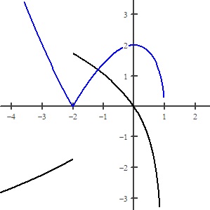
While not required for the exam, you could use a grapher in implicit mode to graph the relation. Without the y > 0 restriction the graph consists of two seemingly parallel graphs similar to a sine graph. They are not sine graphs.

Ideas for exploring this question:

Using a graphing utility that allows you to use sliders. Replace the -6 by a variable that will allow you to see all the members of this family using a slider.
If the slider value is between -1/8 and 0 the graph no longer looks the same. Explore with this.
If the slider value is < -1/8 there is no graph. Why?
Explain why these are not sine graphs. (Hint: Use the quadratic formula to solve for y):

$\displaystyle y=\frac{{\sin (x)\pm \sqrt{{{{{(\sin (x))}}^{2}}+48}}}}{4}$ .

Part (a): There is not much you can change in this part. Ask for the derivative of a different implicit relation. You may use other questions of this type. Good Question 17, 2004 AB 4, 2016 BC 4 (parts a, b, and c are suitable for AB).

Discussion and ideas for adapting this question:

Ask for the first derivative without showing student the answer.
Find the derivative from the expression when first solved for y. Show that this is equal to the given derivative.

Part (b): An easy, but important question: write the equation of the tangent line at a given point. Writing the equation of a line shows up somewhere on the exam every year. As always, use the point-slope form.

Discussion and ideas for adapting this question:

Use a different point.

Part (c): Students were asked to find the point in a specific interval where the tangent line is horizontal.

Discussion and ideas for adapting this question:

By enlarging the domain find other points where the tangent line is horizontal. (Not likely to be asked on the exam, but good exercise.)
Using y < 0 find where the tangent line is horizontal. (Not likely to be asked on the exam, but good exercise.)
Determine if the two parts of the graph are “parallel.”
Determine if the two parts of the graph are congruent to $y=\tfrac{1}{4}\sin \left( x \right)$ .

Part (d): Students were asked to determine if the point found in the previous part was a relative maximum, minimum or neither, and to justify their answer.

Discussion and ideas for adapting this question:

Have students justify using the Candidates’ test (closed interval test).
Have students justify using the first derivative test.
Have students justify using the second derivative test.
Ask the same question for the branch with y < 0.

Having students justify local extreme values by all three methods is good practice any time there is a justification required. Depending on the problem, it may not be possible to use all three. Discuss why; discuss how to decide which is the most efficient for each problem.

Next week 2021 AB 6.

I would be happy to hear your ideas for other ways to use this question. Please use the reply box below to share your ideas.

Good Question 17

Posted on January 21, 2020 by Lin McMullin

A common question in (older?) textbooks is to give students a function or relation and have them graph it without technology (because in the old days technology was not available). Students had to find all the appropriate information without hints or further direction: they were supposed to know what to do and do it.

AP exam questions, for legitimate and understandable reasons, do not ask for as complete an analysis. Rather, they ask students to find specific information about the function or its graph (extreme values, points of inflection, etc.). For the same legitimate and understandable reason many of the features are not considered; the other concepts are tested on different questions.

I think that the full-analysis-from-scratch approach, while not appropriate for an AP exam question, has its merits. The big difference is that students need to be creative in their investigation; not just focus on a few items pointed to by the question.

With that in mind, let’s consider the following question asked three ways.

A very general form

Consider the relation ${{x}^{3}}+3{{x}^{2}}+{{y}^{2}}=4$ . Discuss the graph of the relation giving reasons for your conclusions. Include a brief mention of any unproductive paths you followed and what you learned from them.

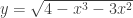
A more directed investigation

Consider the relation ${{x}^{3}}+3{{x}^{2}}+{{y}^{2}}=4$ . Find its extreme values and any asymptotes, and vertical tangents (if any). Discuss in detail the appearance of the graph near x = –2 and discuss the slopes in that area. Explain how you arrived at your results.

Closer to an AP style form. The function here is the top half of the function above.

Consider the function $y=\sqrt{{4-{{x}^{3}}-3{{x}^{2}}}}$ .

(a) Find the local maximum and minimum values of the function. Justify your answer.

(b) Where does the function had a vertical asymptote? Justify your answer.

(c) Find $\underset{{x\to -2-}}{\mathop{{\lim }}}\,\frac{{dy}}{{dx}}$ and $\underset{{x\to -2+}}{\mathop{{\lim }}}\,\frac{{dy}}{{dx}}$ . What does this say about the graph?

The real question is can you ask it the first way?

Here is my solution to the first form; this will also give the answers to the other forms. After the solution, I’ll discuss some ideas on how to score such a solution.

Solution

The graph of the relation ${{x}^{3}}+3{{x}^{2}}+{{y}^{2}}=4$ . is shown in figure 1.

Figure 1

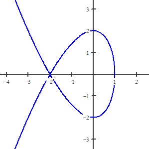
The domain of the function is $x\le 1$ . Values greater than 1 will make the left side of the equation greater than 4 regardless of the value of y. The range of the relation is all real numbers.

The function is symmetric to the x-axis since substituting (–y) for y will give the same expression. The equation of the top half is $y=\sqrt{{4-{{x}^{3}}-3{{x}^{2}}}}$ and the lower half is $y=-\sqrt{{4-{{x}^{3}}-3{{x}^{2}}}}$

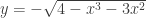
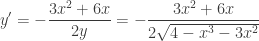
The derivative for the top half is $\displaystyle {y}'=-\frac{{3{{x}^{2}}+6x}}{{2y}}=-\frac{{3{{x}^{2}}+6x}}{{2\sqrt{{4-{{x}^{3}}-{3{x}^{2}}}}}}$ by implicit differentiation or by differentiating the equation for the top half.

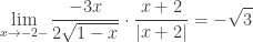
$y'\left( x \right)$ does not exist at x = 1 specifically, $\displaystyle \underset{{x\to 1-}}{\mathop{{\lim }}}\,{y}'\left( x \right)=-\infty$ . Therefore, the line x = 1 is a vertical tangent. By symmetry for the lower part of the graph $\displaystyle \underset{{x\to 1-}}{\mathop{{\lim }}}\,{y}'\left( x \right)=+\infty$ . And x = 1 is its vertical asymptote as well. The slope of the original relation changes from positive to negative at x = 1 by going not through zero but from $-\infty$ to $+\infty$ .

${y}'\left( x \right)=0$ when x = 0 and when x = –2. At (0, 2) the derivative changes from positive to negative; this is a local maximum point by the first derivative test. The lower half has a local minimum point at (0, –2) by symmetry.

At (–2, 0) the derivative is an indeterminate form of the type 0/0.

False step: At first, I thought this meant that the two sides were tangent to the line x = –2 making the point (–2, 0) on the top half a cusp. I tried to see if this was true by graphing in a very narrow window. This did not show anything: the graph looked on zooming in, like an absolute value graph. It turned out that an absolute value was involved.

I then made a table of values for the derivative near the point and found that the values appeared to be approaching a number near –1.7 from the left and near +1.7 from the right. I started thinking maybe $\displaystyle \sqrt{3}$ .

Then I changed the constants to parameters and played with the sliders on Desmos (here). With a slight change in the constants the graph appeared to have a nice rounded local minimum near x= –2. Other values showed two separate pieces with vertical tangents near x= –2. This confused me even more.

Next, I did what I should have done earlier: I graphed the top half and its derivative (figure 2):

Figure 2. The top half in blue and its derivative in black.

The derivative has a finite jump discontinuity at x = –2. I remembered seeing this kind of thing before and thought it involved an absolute value of some kind. Still confused, I decided to investigate the derivative further (which I also should have done sooner).

The derivative at x = –2 is an indeterminate form of the 0/0 type. This means that by substituting you get an expression that really doesn’t help; you may still evaluate the limit (remember derivatives are limits) by other methods. Factoring the derivative (using synthetic division on the radicand) gives

$\displaystyle {y}'\left( x \right)=-\frac{{3x\left( {x+2} \right)}}{{2\sqrt{{{{{\left( {x+2} \right)}}^{2}}\left( {1-x} \right)}}}}=-\frac{{3x\left( {x+2} \right)}}{{2\sqrt{{{{{\left( {x+2} \right)}}^{2}}}}\sqrt{{1-x}}}}=-\frac{{3x}}{{\sqrt{{1-x}}}}\frac{{x+2}}{{\left| {x+2} \right|}}$

And now we see that

$\displaystyle \underset{{x\to -2-}}{\mathop{{\lim }}}\,\frac{{-3x}}{{2\sqrt{{1-x}}}}\cdot \frac{{x+2}}{{\left| {x+2} \right|}}=-\sqrt{3}$ and $\displaystyle \underset{{x\to -2+}}{\mathop{{\lim }}}\,\frac{{-3x}}{{2\sqrt{{1-x}}}}\cdot \frac{{x+2}}{{\left| {x+2} \right|}}=\sqrt{3}$

This agrees with the derivative’s graph. The top graph (and bottom’s by symmetry) comes to an arrow-like point (sometimes called a node) at (–2, 0). The slope on the left approaches $-\sqrt{3}$ and on the right approaches $+\sqrt{3}$ .

______________________

I admit I’ve had a few more years of experience with this sort of thing that a first-year calculus student. I expect this would be difficult for most students who have never seen a question like this, so working up to it with simpler questions is how to start.

In grading this sort of question, you need to consider:

If the student found and justified all the pertinent features of the graph. If they missed something, what they included may still be pretty good. For example, I would not expect a student to the use the word “node,” so omitting it should not be held against them and using it may call for praise.
The things they (and I) may have overlooked or things they considered that were unnecessary or even wrong.
Their overall approach. This last may be the most important part. Including their missteps and unproductive paths is important and should, I think, receive credit. After all, they did not know the path would be unproductive until they followed it a way. Hopefully, they made some missteps and learned something from them. That’s what investigating something in math entails.

I would be happy to hear if you tried this or something similar and so would the other readers of this blog. Please use the “Comment” button below to share your thoughts.

Local Linearity

Posted on August 28, 2018 by Lin McMullin

If you use your calculator or graphing program and zoom-in of the graph of a function (with equal zoom factors in both directions), the graph eventually looks like a line: the graph appears to be straight. This property is called Local Linearity. The slope of this line is the number called the derivative. (There are exceptions: if the graph never appears linear, then no derivative exists at that point.) Local Linearity is the graphical manifestation of differentiability.

To find this slope, we need to zoom-in numerically. Zooming-in numerically is accomplished by finding the slope of a secant line, a line that intersects the graph twice near the point we are interested in. Then finding the limit of that slope as the two points come closer to our point. This limit is the derivative. It is also the slope of the line tangent to the function at the point.

While limit is what makes all of the calculus work, people usually think of calculus as starting with the derivative. The first problem in calculus is finding the slope of a line tangent to a graph at a point and then writing the equation of that tangent line. The slope is called the derivative and a function whose derivative exists is said to be differentiable.

This week’s posts start with local linearity and tangent lines. They lead to the difference quotient and the equation of the tangent line.

Local Linearity I

Local Linearity II Working up to difference quotient. The next post explains this in more detail.

Tangent Lines approaching difference quotients on calculator by graphing tan line.

Next week: Difference Quotients.

Revised from a post of August 29, 2017

Difference Quotients

Posted on September 5, 2017 by Lin McMullin

Difference quotients are the path to the definition of the derivative. Here are three posts exploring difference quotients.

Difference Quotients I The forward and backward difference quotients

Difference Quotients II The symmetric difference quotient and seeing the three difference quotients in action. Showing that the three difference quotients converge to the same value.

Seeing Difference Quotients Expands on the post immediately above and shows some numerical and graphical approaches using calculators and Desmos.

Tangents and Slopes You can use this Desmos app now to preview some of the things that he tangent line can tell us about the graph of a function or save (or reuse) it for later when concentrating on graphs. Discuss slope in relation to increasing, decreasing, concavity, etc.

At Just the Right Time

Stamp out Slope-intercept Form

Who’d a thunk it?

Posted on July 18, 2017 by Lin McMullin

Cubic Symmetry

Some things are fairly obvious. For example, if you look at the graphs of a few cubic equations, you might think that each is symmetric to a point and on closer inspection the point of symmetry is the point of inflection.

This is true and easy to prove. You can find the point of inflection, and then show that any point a certain distance horizontally on one side is the same distance above (or below) the point of inflection as a point the same distance horizontally on the other side is below (or above). Another way is to translate the cubic so that the point of inflection is at the origin and then show the resulting function is an odd function (i.e. symmetric to the origin).

But some other properties are not at all obvious. How someone thought to look for them is not even clear.

Tangent Line.

If you have cubic function with real roots of x = a, x = b, and x = c not necessarily distinct, if you draw a tangent line at a point where x is the average of any two roots, x = ½(a + b), , then this tangent line intersects the cubic on the x-axis at exactly the third root, x = c. Here is a Desmos graph illustrating this idea.

Here is a proof done with a CAS. The first line is a cubic expressed in terms of its roots. The third line asks where the tangent line at x = m intersects the x-axis. The last line is the answer: x = c or whenever a = b (i.e. when the two roots are the same, in which case the tangent line is the x-axis and of course also contains x = c.

Areas
Even harder to believe is this: Draw a tangent line anywhere on a cubic. This tangent will intersect the cubic at a second point and the line and the cubic will define a region whose area is A1. From the second point draw a tangent what intersects the cubic at a third point and defines a region whose area is A2. The ratio of the areas A2/A1 = 16. I have no idea why this should be so, but it is.

Here is a proof, again by CAS: The last line marked with a square bullet is the computation of the ratio and the answer, 16, is in the lower right,

And if that’s not strange enough, inserting two vertical lines defines other regions whose areas are in the ratios shown in the figure below.

Who’d a thunk it?

Tangent Lines

Posted on August 23, 2016 by Lin McMullin

Second in the Graphing Calculator/Technology series

This graphing calculator activity is a way to introduce the idea if the slope of the tangent line as the limit of the slope of a secant line. In it, students will write the equation of a secant line through two very close points. They will then compare their results in several ways.

Begin by having the students graph a very simple curve such as y = x² in the standard window of their calculator. Then TRACE to a point. Students will go to different points, some to the left and some to the right of the origin. ZOOM IN several times on this point until their graph appears linear (discuss local linearity here). To be sure they are on the graph push TRACE again. The coordinates of their point will be at the bottom of the screen; call this point (a, b). Return to the home screen and store the values to A and B (click here for instructions on storing and recalling numbers).

Return to the graph and push TRACE again to be sure the cursor is on the graph. Move the TRACE cursor one or two pixels away from the first point in either direction. This new point is (c, d). Return to the home screen and store the coordinates to C and D.

Enter the equation of the line through the two points on the equation entry screen in terms of A, B, C, and D. Zoom Out several times until you have returned to the original window..

Exploration 1: Have students compare and contrast their graphs with several other students and discuss their observations. (Expected observations: the lines appear tangent at each students’ original point)

Exploration 2: Ask student to compute the slope of the line through their points, again using A, B, C, and D. Collect each student’s x-coordinate, A, and their slope and enter them in list is your calculator so that they can be projected.

Study the two lists and discuss the relation is any. (Expected observations: the slope is twice the x-coordinate.) Can you write an equation of these pairs? (Expected result: y = 2x)

Finally, plot the points on the calculator using a square window. Do the points seem to lie on the line y =2x?

Extensions:

Try the same activity with other functions such as y = (1/3)x³, y = x³, or y = x⁴. Anything more difficult will still result in a tangent line, but the numerical relationship between x and the slope will probably be too difficult to see. You may also consider y = sin(x) or y = cos(x). Again, the numerical work in Exploration 2, will be too difficult to see, but on graphing the points the result may be obvious. For y = sin(x), return to the list and add a column with the cosines of the x-values. Compare these with the slopes.

At Just the Right Time

Posted on September 12, 2013 by Lin McMullin

This is about a little problem that appeared at just the right time. My class had just learned about derivatives (limit definition) and the fact that the derivative is the slope of the tangent line. But none of that was really firm yet. I had assigned this problem for homework:¹

Find f (3) and f ‘ (3), assuming that the tangent line to y = f (x) at a = 3 has equation y = 5x + 2

To solve the problem, you need to realize that the tangent line and the function intersect at the point where x = 3. So, f (3) was the same as the point on the line where x = 3. Therefore, f (3) = 5(3) + 2 = 17.

Then you have to realize that the derivative is the slope of the tangent line, and we know the tangent line’s equation and we can read the slope. So f ‘ (3) = 5

In my previous retired years, I wrote a number of questions for several editions of a popular AP Calculus exam review book.² I found it easy to write difficult questions. But what I was after was good easy questions; they are more difficult to write. One type of good easy question is one that links two concepts in a way that is not immediately obvious such as the question above. I am always amazed at the good easy questions on the AP calculus exams. Of course, they do not look easy, but that’s what makes them good.

Now a month from now this question will not be a difficult at all – in fact it did not stump all of my students this week. Nevertheless, appearing at just the right time, I think it did help those it did stump, and that’s why I like it.

______________________

² These review books are published by D&S Marketing Systems, Inc. Website

Teaching Calculus

The pleasure lies not in discovering the truth, but in searching for it.

Tag Archives: tangent line

Adapting 2021 AB 5

2021 AB 5

Good Question 17

Solution

Local Linearity

Difference Quotients

Who’d a thunk it?

Tangent Lines

At Just the Right Time

2021 AB 5

Share this:

Like this:

Solution

Share this:

Like this:

Share this:

Like this:

Share this:

Like this:

Share this:

Like this:

Share this:

Like this:

Share this:

Like this: