Quick Notes

Two quick notes:

First, I’ve added a new page with activities and explorations I have collected and used with students and in my summer institutes. Some are formatted as handouts (a/k/a worksheets) and others are black line masters for game type activities. You can find them under the “Resources” tab on the top line menu (direct link). I will be looking through my files for more, so check back now and then. Hope you find them helpful.

Second: last year I reviewed an iPad app called A Little Calculus. This app demonstrates graphically nearly all the concepts of AB and BC Calculus. It is quite easy to use and a quick way to prepare and present good visual examples for your class. Your students may also use it to explore on their own or with directions from you. The app has recently been updated to allow you to save and recall your own examples. This is a helpful improvement allowing you to prepare things in advance or reuse set-ups in later classes. Also, two new topics have been added – Logistic Growth and the Derivative of Exponential Functions. If you are not familiar with it, take a look.

Advertisement

…but what does it look like?

It will soon be time to teach about finding the volumes of solid figures using integration techniques. Here is a list of links to posts that will help your students what these figures look like and how they are generated.

Visualizing Solid Figures 1 Here are ideas for making physical models of solid figures. These make good projects for students.

A Little Calculus is an iPad app that does an excellent job in helping students visualize many of the concepts of the calculus. Volumes with regular cross section, disk method, washer method, cylindrical shells are all illustrated.

The first illustrations show square cross sections on a semicircular base. The base is in the lower part and the solid in the upper. By using the plus and minus button (lower right) you can increase or decrease the number of sections in real time and see the figures change. The upper figure may be rotated by moving your finger on the screen.

The illustration below shows a washer situation.


The following older posts show how to use Winplot to generate and explore solid figures. Unfortunately, Winplot seems to have gone out of favor. I’m not sure why; it is one of the best. I still use it and like it. You may download Winplot here for free (PC only).

Visualizing Solid Figures 2 This post demonstrates how to use Winplot to generate solids with regular cross sections and solids of rotation.

Visualizing Solid Figures 3 The washer method is illustrated using Winplot. These post all relate to finding volumes by washers: Subtract the Hole from the Whole and Does Simplifying Make Things Simpler?

Visualizing Solid Figures 4 Using Winplot to see the method cylindrical shells. Note that this method is not tested on either the AB or BC Calculus exams, so you do not have to teach it. Many teachers present this topic after the exams are given. As a footnote you may also find Why You Never Need Cylindrical Shells interesting. (However, this is not the reason it is not tested on the AP Calculus exams.)

Visualizing Solid Figures 5 An exercise demonstrating how “half” can mean different things and shows that how the figures are generated makes a difference.

“A Little Calculus”

A Little Calculus is an app for iPad and iPhones. While I don’t usually do product reviews, I think this one is so good that I am making an exception.

There are many good websites that illustrate calculus concepts. Many of them, however, do not allow teachers to enter their own examples; they must use the built-in ones. A Little Calculus is an exception.

A Little Calculus contains over 75 demonstrations of calculus and calculus related concepts, and also three graphing calculators (Cartesian, Parametric, and Polar). Each demonstration can be fully edited to any function and conditions by the user. The topics cover precalculus, limits and continuity, Differential Calculus, Integral Calculus, Sequences and Series, Parametric Curves, and Multivariable Calculus. A full list of the concepts included is at the end of this post. The app is available in the App Store; the price is (only) $0.99. Link.

Each topic has an information screen (circled I in the upper right of the screen) that includes (1) “How To” explaining how to input your example and how to use the features specific to that demonstration. (You should read this the first time you use each topic because some features may not be obvious.), (2) “Background” a textbook-like page that explains in detail the mathematics demonstrated, and (3) “Examples” discussing one or more examples of the concept.

The set-up screen (chevron upper right) allows the user to enter the example they want. This then changes to a pull-down screen. The screenshot below is the set-up screen for “The Area Under a Curve” demonstration. Note the Riemann rectangles available from the set-up screen.

The resulting graph is shown next for 3 right Riemann sum rectangles. By clicking on the “+” or “-“ in the bottom right, you can increase or decrease the number of rectangles one at a time; by holding the “+” sign the number increases rapidly to demonstrate n → ∞. The upper and lower limits may be specified on the set-up screen or be dragged from the graph. The current area of the rectangles is shown in the lower left.

The next illustration shows the “Disk Method” section. The lower graph shows the individual rectangles; the upper shows the 6 rectangles rotated around the line y = –1/2. The “+” button increases the number of rectangles.

This shot shows 150 rectangles; the upper graph has been rotated slightly – this is accomplished in real time by dragging your finger across the screen. All three-dimensional graphs may be moved in this manner.

I could go on …

The one slight drawback is that the input screen does not allow the user to enter parentheses. The parentheses are entered correctly by selecting what is to be enclosed and then tapping the next operation button. This leads to some strange looking expressions such as sin(x)2 instead of (sin(x))2. The expressions are interpreted correctly, but the strange look may confuse some students. It would be easier to type them yourself as usual. Not a big problem.

An effective way to use this app if for the teacher to project a demonstration and discuss the various ideas he or she wishes to discuss. Tapping the screen with two fingers toggles a pointer; this is useful for working on-line with students who cannot see where you are pointing otherwise. Students could use the app to investigate on their own.

UPDATE (August 18,2022) A new feature has been added: you may now save and recall your own example(s) instead of having to reenter them each time. Handy for preparing demonstrations ahead of time or having students prepare their own examples.

Also, two new topics have been added: Logistic growth and the derivative of an exponential function.

Here is a list of the other topics included:


Update 8-18-2022


Spiral Slide Rule

As I wrote last week, I found an old spiral slide rule last summer. It is about the size of a rolling pin and in fact has a handle like a rolling pin’s at the bottom. The device consists of a short wide cylinder that slides around, and up or down on a longer thin cylinder.

The short wide cylinder has a spiral common (base 10) logarithm scale starting at the top at the 100 mark after the words “slide rule” (see Figure 3). The scale runs around the cylinder 50 times ending precisely under the starting mark. By my measurement the scale is about 511 inches or 42.6 feet long. (1.30 meters). The scale is marked for 4 digits reading with a 5th digit that can be reasonably estimated. (By way of comparison, the common 10-inch slide rule scale discussed last week allows for 2 digits reading with the third digit estimated.) These are the mantissas of the common logarithms from 1 at the zero point (since log (1) = 0) to 1.0 (log (10) = 1) at the lower end.

The thin cylinder is marked with several formulas and other information including a table of natural sines from 0 to 45 degrees, from which you can have the value of any trig function if you’re clever enough. This cylinder is not used for calculations; it is there to allow the wider cylinder to move.

There are also two pointers. The shorter one is attached to the bottom and fixed. The cylinder is moved into position for this pointer. The longer pointer is attached to the thin cylinder and can be moved to the position needed – up, down left or right. Both the top end and the bottom end of the long pointer may be used. The pointers are made to slide past each other if necessary. If the long pointer covers the number needed the other side of it may be used instead (just don’t switch back-and-forth in the same computation).

Here is how it works. For the multiplication problem 15.115 x 439.65.

For the moment we ignore the decimal points.

  1. The top, “T” shaped, pointer is moved to the start value after “Slide rule.”
  2. The bottom pointer is first set at 15115 (the 151 is marked, the next 1 is the first mark following 151 and the 5 is estimated. See Figure 3 (Click to enlarge). The distance between the two measured almost 9 times around the cylinder is log (1.5115)
  3. Next the cylinder is moved without disturbing the pointers so that the top pointer is at 4.3965 and again estimating the last digit. Figure 4 upper long pointer.
  4. The product is at the fixed pointer: 6.645 Figure 4 lower pointer.
  5. Finally, we put the decimal in the proper place. The product is 6645.
  6. The full value is 6645.30975 by calculator. So the answer is correct to 4 digits, good enough for most practical work.

By moving the top pointer to log (4.3965) and using the pointers to add to it log (1.5115) we have performed the calculation log (1.5115) + log (4.3965) = log (1.5115. x 4.3965) = log (6.645)

To divide the procedure is reversed.  \frac{{6645}}{{439.65}}

  1. Set the fixed pointer to the dividend and move the top pointer to one of the divisors. (Figure 4)
  2. Without moving the pointers, move the cylinder so the top pointer is at 1.
  3. The quotient is at the fixed pointer (Figure 3)
  4. Adjust the decimal point for the quotient: 15.115.

If the cylinder is moved so that the pointer is off the bottom of the cylinder, the bottom pointer is used instead of the top. (This is the reason it is directly below the top pointer.)

If this seems like a lot of trouble, it is. But remember, a working computer was not available until near the end of World War II and filled a room. Electronic calculators were not available until around 1970. Computations before then were done by hand or with logarithms.

When I was in college in the early 1960s, I worked for an engineer on my summer vacations. My boss had and occasionally used a large table of logarithms. Large, as in a whole book! As I recall, it was good without interpolating for at least 6 digits accuracy. I used a large desktop mechanical calculator that had a hand crank to do calculations. Hence the term “crank out the answer.”

As for teaching: In those old days before about 1970, you spent 3 to 4 weeks in Algebra 2 teaching students how to use logarithm table and compute with logarithms. I gave that up when the students started using calculators to do the adding and subtracting of their logarithms.

The one advantage of the spiral slide rule is that it doesn’t need batteries!

Happy Holidays!

Slide Rules

Last summer I bought myself a new calculator. Well, it’s actually an old calculator manufactured in 1914 (if I’m reading the correct information engraved on it). It is called a Fuller Spiral Slide Rule.

Before looking at that, I’ll try to explain how the more standard (flat) slide rule works. Next week, I show you the spiral slide rule. Hopefully, you and your students will find this historical note interesting and it will show you how logarithms used to be used. Slide rules were the standard for mathematics, science, and engineering students from the 19th century up to about 1970 when electronic calculators took over. Everyone in STEM fields used them, there was no other choice.

If you were in high school after 1970 you probably never had to learn how to use a slide rule, but you’re probably heard of them.

Let’s look at the standard slide rule. You can find a working virtual model here. (The model doesn’t work on an iPad; you’ll have to use it on a computer.) This It is called a 10-inch slide rule because the scales are 10 inches long.

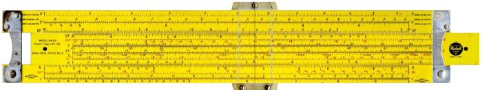
You can move the slide (center section) with your mouse. You can also move the piece withthe screws top and bottom, called the cursor. The cursor is used to read non-adjacent scales and scales on the other side. (Click in the upper right to see the other side). In a real slide rule the slide can be turned over and used with the other side if necessary.

The slide rule only gives the digits of the answer. The decimal point must be determined separately.

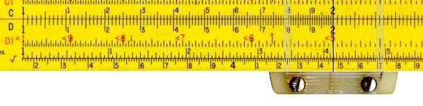
The main scales are the C and D scales. These scales are identical and are marked so that the distance from the left end is the mantissa of the common (base 10) logarithm of the number on the scale. The mantissa is the decimal part of the logarithm. The numbers on the C and D scales are all between 0  (= log (1)) and 1 (= log(10)). The scales allow for 3-digit accuracy on the left up to 4 where the spacing allows for only 2-digits. In each case an extra digit may be estimated.

To multiply: slide the 1 on the C scale until it is above the first factor on the D scale. Then find the second factor on the C scale and the number below it on the D scale is the product. Figure 1 shows the computation of 4 x 2 = 8. Remember the distance from the ends are really logarithms, so what you are really doing is log (4) + log (2) = log (4 X 2) = log (8).

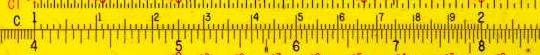
Figure 1: Showing 4 x 2 = 8

Other products may also be seen such as 4 x 1.5 = 6, or 40 x 17.5 = 700, etc.

If the second factor is off the right end of the scale; put the 1 on the right side of the C scale over the first factor and the product will be under the second factor. The second figure shows 4 x 5 = 20 (and other products with 4 as a factor). Remember you need to properly place the decimal point.

Figure 2: Showing 4 x 5 = 20

Division is just the reverse: 8 divided by 2 is done by putting the 2 over the 8 and reading the quotient, 4, under the 1 on the C scale. (See figure 1 again). The scales are interchangeable so you could also put the 8 over the 2 (looks better) and find the quotient on the C scale over the 1 on the D scale. Can you find 60 divided by 15 = 4? On figure 2 you can see 2 divided by 5 = 0.4 or 2800 divided by 0.07 = 40,000.

Chain computations can be done by using the cursor to mark (without reading) one answer and then move on to the next, either multiplying or dividing.

The other scales give other functions. The lower scale marked with a radical sign gives square roots. Move the cursor to 2 and read the square root of two (1.414) on the top part of the scale and the square root of 20 (4.472) on the lower part.

Figure 3: Showing \displaystyle \sqrt{2}\approx 1.414 or \displaystyle \sqrt{{20}}\approx 4.47

The S scale gives the sines and cosines of numbers in degrees. Reading from the left the black numbers are for sines and reading from the right the red numbers are for cosines. See figure 3. The cursor is on 60/30 for the sin(30) = cos(60) the value is on the C scale 0.5 (remember you need to supply the decimal). Reading in the other direction the sin-1(0.5) = 30 or cos-1(0.5) = 60.

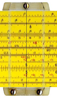
Figure 4: Showing sin(30) = 0.5 = cos(60) or arcsin(0.5) = 30 or arccos(0.5) = 60.

The CF and DF scales are “folded” at \displaystyle \pi to make multiplying by \displaystyle \pi easier. Computations are done the same way. The CI, DI, CIF, and DIF give the reciprocal (I for inverse) and are read right to left.  T is for tangents a double scale from 0 to 45 degrees on the top and 45 degrees on up at the bottom. I’ll leave the others for you to research.

So, that’s today’s history lesson. Next week, the Spiral Slide Rule – a little more complicated, but a lot more accurate.
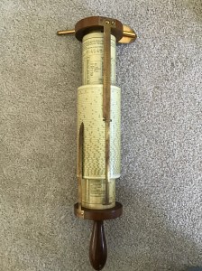
Spiral Slide Rule


An Exploration in Differential Equations

This is an exploration based on the AP Calculus question 2018 AB 6. I originally posed it for teachers last summer. This will make, I hope, a good review of many of the concepts and techniques students have learned during the year. The exploration, which will take an hour or more, includes these topics:

  • Finding the general solution of the differential equation by separating the variables
  • Checking the solution by substitution
  • Using a graphing utility to explore the solutions for all values of the constant of integration, C
  • Finding the solutions’ horizontal and vertical asymptotes
  • Finding several particular solutions
  • Finding the domains of the particular solutions
  • Finding the extreme value of all solutions in terms of C
  • Finding the second derivative (implicit differentiation)
  • Considering concavity
  • Investigating a special case or two

I also hope that in working through this exploration students will learn not so much about this particular function, but how to use the tools of algebra, calculus, and technology to fully investigate any function and to find all its foibles.

The exploration is here in a PDF file. Here are the solutions.

As always, I appreciate your feedback and comments. Please share them with me using the reply box below.


The College Board is pleased to offer a new live online event for new and experienced AP Calculus teachers on March 5th at 7:00 PM Eastern.

I will be the presenter.

The topic will be AP Calculus: How to Review for the Exam:  In this two-hour online workshop, we will investigate techniques and hints for helping students to prepare for the AP Calculus exams. Additionally, we’ll discuss the 10 type questions that appear on the AP Calculus exams, and what students need know and to be able to do for each. Finally, we’ll examine resources for exam review.

Registration for this event is $30/members and $35/non-members. You can register for the event by following this link: http://eventreg.collegeboard.org/d/xbqbjz


Continuity

Karl Weierstrass (1815 – 1897) was the mathematician who (finally) formalized the definition of continuity. Included in that definition was the epsilon-delta definition of limit. This definition has been pulled out, so to speak, and now is usually presented on its own. So, which came first – continuity or limit? The ideas and situations that required continuity could only be formalized with the concept of limit. So, looking at functions that are or are not continuous helps us understand what limits are and why we first need them.

In the ideal world, students would have plenty of work with continuous and not continuous functions before starting the calculus. The vocabulary and notation, if not the formal definitions, would be used as early as possible. Then when students got to calculus, they would know the ideas and be ready to formalize the ideas.

The Intermediate Value Theorem (IVT) is an important property of continuous functions.

Using the definition of continuity to show that a function is or is not continuous at a point is a common question of the AP exams, as is the IVT.

Continuity The definition of continuity.

Continuity Should continuity come before limits?

From One Side or the Other One-sided limits and one-sided differentiability

How to Tell Your Asymptote from a Hole in the Graph  From the technology series. Showing holes and asymptotes on a graphing calculator.

Fun with Continuity Defined everywhere and continuous nowhere. Continuous only at a single point.

Theorems The Intermediate Value Theorem (IVT) and suggestions on teaching theorems.

Intermediate Weather  Using the IVT

Right Answer – Wrong Question Continuity or continuity “on its domain”?


Revised from a post of August 22, 2017