Unit 9 – Parametric Equations, Polar Coordinates, and Vector-Valued Functions

Posted on January 11, 2022 by Lin McMullin

Unit 9 includes all the topics listed in the title. These are BC only topics (CED – 2019 p. 163 – 176). These topics account for about 11 – 12% of questions on the BC exam.

Comments on Prerequisites: In BC Calculus the work with parametric, vector, and polar equations is somewhat limited. I always hoped that students had studied these topics in detail in their precalculus classes and had more precalculus knowledge and experience with them than is required for the BC exam. This will help them in calculus, so see that they are included in your precalculus classes.

Topics 9.1 – 9.3 Parametric Equations

Topic 9.1: Defining and Differentiation Parametric Equations. Finding dy/dx in terms of dy/dt and dx/dt

Topic 9.2: Second Derivatives of Parametric Equations. Finding the second derivative. See Implicit Differentiation of Parametric Equations this discusses the second derivative.

Topic 9.3: Finding Arc Lengths of Curves Given by Parametric Equations.

Topics 9.4 – 9.6 Vector-Valued Functions and Motion in the plane

Topic 9.4 : Defining and Differentiating Vector-Valued Functions. Finding the second derivative. See this A Vector’s Derivatives which includes a note on second derivatives.

Topic 9.5: Integrating Vector-Valued Functions

Topic 9.6: Solving Motion Problems Using Parametric and Vector-Valued Functions. Position, Velocity, acceleration, speed, total distance traveled, and displacement extended to motion in the plane.

Topics 9.7 – 9.9 Polar Equation and Area in Polar Form.

Topic 9.7: Defining Polar Coordinate and Differentiation in Polar Form. The derivatives and their meaning.

Topic 9.8: Find the Area of a Polar Region or the Area Bounded by a Single Polar Curve

Topic 9.9: Finding the Area of the Region Bounded by Two Polar Curves. Students should know how to find the intersections of polar curves to use for the limits of integration.

Timing

The suggested time for Unit 9 is about 10 – 11 BC classes of 40 – 50-minutes, this includes time for testing etc.

Previous posts on these topics:

Parametric and Vector Equations

Implicit Differentiation of Parametric Equations

A Vector’s Derivatives

Adapting 2012 BC 2 (A parametric equation question)

Polar Curves

Polar Equations for AP Calculus

Extreme Polar Conditions

Visualizing Unit 9 Desmos Demonstrations for Polar, Vector and Parametric Curves

Implicit Differentiation of Parametric Equations

Posted on October 31, 2021 by Lin McMullin

I’ve never liked memorizing formulas. I would rather know where they came from or be able to tie it to something I already know. One of my least favorite formulas to remember and explain was the formula for the second derivative of a curve given in parametric form. No longer.

If $\displaystyle y=y(t)$ and, $\displaystyle x=x(t)$ then the traditional formulas give

$\displaystyle \frac{{dy}}{{dx}}=\frac{{dy/dt}}{{dx/dt}}$ , and

$\displaystyle \frac{{{{d}^{2}}y}}{{d{{x}^{2}}}}=\frac{{\frac{d}{{dt}}\left( {\frac{{dy}}{{dx}}} \right)}}{{\frac{{dx}}{{dt}}}}$

It is that last part, where you divide by $\displaystyle {\frac{{dx}}{{dt}}}$ , that bothers me. Where did the $\displaystyle {\frac{{dx}}{{dt}}}$ come from?

Then it occurred to me that dividing by $\displaystyle {\frac{{dx}}{{dt}}}$ is the same as multiplying by $\displaystyle {\frac{{dt}}{{dx}}}$

It’s just implicit differentiation!

Since $\displaystyle \frac{{dy}}{{dx}}$ is a function of t you must begin by differentiating the first derivative with respect to t. Then treating this as a typical Chain Rule situation and multiplying by $\displaystyle {\frac{{dt}}{{dx}}}$ gives the second derivative. (There is a technical requirement here that given $\displaystyle x=x(t)$ , then its inverse $\displaystyle t={{x}^{{-1}}}\left( x \right)$ exists.)

In fact, if you look at a proof of the formula for the first derivative, that’s what happens there as well:

$\displaystyle \frac{d}{{dx}}y(t)=\frac{{dy}}{{dt}}\cdot \frac{{dt}}{{dx}}=\frac{{dy/dt}}{{dx/dt}}$

The reason you do it this way is that since x is given as a function of t, it may be difficult to solve for t so you can find dt/dx in terms of x. But you don’t have to; just divide by dx/dt which you already know.

Here is an example for both derivatives.

Suppose that $\displaystyle x={{t}^{3}}-3$ and $\displaystyle y=\ln \left( t \right)$

Then $\displaystyle \frac{{dy}}{{dt}}=\frac{1}{t}$ and $\displaystyle \frac{{dx}}{{dt}}=3{{t}^{2}}$ and $\displaystyle \frac{{dt}}{{dx}}=\frac{1}{{3{{t}^{2}}}}$

Then $\displaystyle \frac{{dy}}{{dx}}=\frac{1}{t}\cdot \frac{{dt}}{{dx}}=\frac{1}{t}\cdot \frac{1}{{3{{t}^{2}}}}=\frac{1}{3}{{t}^{{-3}}}$

And $\displaystyle \frac{{{{d}^{2}}y}}{{d{{x}^{2}}}}=\left( {\frac{d}{{dt}}\left( {\frac{{dy}}{{dx}}} \right)} \right)\cdot \frac{{dt}}{{dx}}=\left( {-{{t}^{{-4}}}} \right)\cdot \left( {\frac{1}{{3{{t}^{2}}}}} \right)=-\frac{1}{{3{{t}^{6}}}}$

Yes, it’s the same thing as using the traditional formula, but now I’ll never have to worry about forgetting the formula or being unsure how to explain why you do it this way.

Revised: Correction to last equation 5/18/2014. Revised: 2/8/2016. Originally posted May 5, 2014.

Adapting 2021 BC 5

Posted on August 10, 2021 by Lin McMullin

Eight of nine. We continue our study of the 2021 free-response questions. We will look at ways to adapt, expand, and explore this question to help students better understand it and look at other questions that can be asked based on a similar stem.

2021 BC 5

This is a Differential Equation (Type 6) with a Sequence and Series (Type 10) question included. It contains topics from Units 7 and 10 of the current Course and Exam Description (CED). It is not unusual for AP Calculus exam question to include several of the types in my classification and from several of the units from the CED (here units 7 and 10). In addition, the usual solving an initial value problem and a Euler’s Method approximation are included.

The stem for 2021 BC 5 is:

Part (a): Students were asked to write the second-degree Taylor polynomial for the function centered at x = 1 and then use it to approximate f(2). Students should stop after substituting 2 into their polynomial; no arithmetic or simplification is required, and a simplifying mistake will lose a point.

Discussion and ideas for adapting this question:

Ask students to find an expression for the second derivative (implicit differentiation).
Verify that $\displaystyle {f}''\left( 1 \right)=4$
Ask students to find the third-degree polynomial and use it to approximate f(2)

Part (b): Students were required to approximate f(2) using Euler’s method with two steps of equal size.

Discussion and ideas for adapting this question:

After you solve the equation in part (c), ask students to compare the approximations from parts (a) and (b) with the exact value. Neither approximation is very close to the exact value. Discuss why this is so. Consider the slope of the graph near x = 2.
Find a more accurate approximation using 3, 4, or more smaller steps. There are graphing calculator programs that will do the arithmetic. Do not hesitate to use them. Students have already shown they know how to do a Euler’s Method approximation; the point is to understand the situation.

Part (c): Finding the solution of the differential equation by separating the variables is expected in this kind of question. The added twist is that the method of integration by parts is necessary to find one of the antiderivatives.

Discussion and ideas for adapting this question:

Be sure not to skip over removing the absolute value signs. The most efficient way is to realize that at (and near) the initial condition y > 0, so |y| = y. What do you do if y < 0?
There is not much you can do differently here. One thing is to change the initial condition. Try a negative value such as f(1) = –4.
As suggested in (b), compare, and discuss the approximations with the exact value.

Next week we will conclude this series of posts with a look at 2021 BC 6.

I would be happy to hear your ideas for other ways to use this question. Please use the reply box below to share your ideas.

Adapting 2021 AB 6

Posted on July 27, 2021 by Lin McMullin

Six of nine. Continuing the current series of posts, this post looks at the AB Calculus 2021 exam question AB 6. Like most of the AP Exam questions, there is a lot more you can ask based on the stem of this question and a lot of other calculus you can discuss. This series of post offers suggestions as to how to adapt, expand, and use this question to help your students dig deeper and learn more.

2021 AB 6

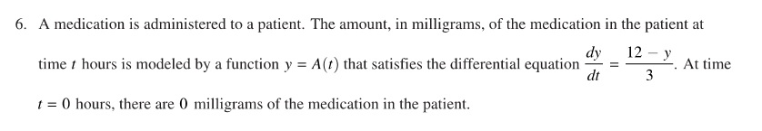
This is a standard Differential Equation (Type 6) question and contains topics mainly from Unit 7 (Differential equations) and a little from Unit 3 (implicit differentiation) of the current Course and Exam Description. A differential equation with an initial condition is given in a context. The main part is the solution of the initial value question with three short other questions included.

The stem for 2021 AB 6 is:

Part (a): A slope field in the first quadrant with no scale on either axis is given. Students are asked to sketch the solution curve starting at the initial condition, the point (0, 0). (I prefer this kind of slope field question to those where students are given a few points and asked to sketch the slope field through them. No one draws slope field by hand; slope field drawn by computers are used to study the approximate shape of the solution and determine its interesting properties as is done here and in part (b)). When drawing slope fields, the sketch should extend to from one border to another and contain the initial condition point.

Discussion and ideas for adapting this question:

Have student sketch solution through one or more different points. Copy the slope field and add the initial condition point somewhere else.
Add an initial point above the horizontal asymptote.
Compare and contrast the solutions drawn through several points.
Ask what the horizontal segments (at y = 12) tells you in the context of the problem.

Part (b): Students are given the limit at infinity for the as yet unknow solution and asked to interpret it in the context of the problem including units of measure.

Discussion and ideas for adapting this question:

Discuss why this is so.
Discuss how to determine the units of the function from the given information.
Discuss how to determine the units of the derivative from the given information.
Discuss how to determine the units of the derivative from the units of the function.
Discuss how to determine the units of the function from the units of the derivative.
Discuss whether the interpretation of the limit makes sense in the context of the question.

Part (c): Students are asked to solve the initial value question using the method of separation of variables.

Discussion and ideas for adapting this question:

Since separation of variables is the only method for solving a differential equation that students are responsible for knowing, there is not much you can do to adapt or change this question.
The initial condition may be substituted immediately after the integration is done the “+ C” is attached, or it may be done later after the expression is solved for y. Show students both method and discuss which is more efficient and which makes more sense to them.
Removing the absolute value signs is another place that may confuse students. While some textbooks suggest using a “ ± “ sign and deciding sign which to use later, the better way is to decide as soon as possible. Ask yourself is the expression enclose by the absolute value signs positive or negative near (at) the initial value. If positive, then the absolute value is replaced by the same expression (as in this question); if negative, then the expression is replaced by its opposite. Then complete the question from there.

Part (d): This part needs careful reading. Students are asked, for a slightly different differential equation, if the rate of change in the amount of medicine is increasing or decreasing at a given time. Therefore, students must find the rate of change of the rate of change (the given derivative): the derivative of the derivative (i.e., the second derivative of the function). This requires implicit differentiation of the derivative using the quotient rule.

Discussion and ideas for adapting this question:

The second derivative has the first derivative as one of its factors. Students may (automatically) substitute the first derivative before simplifying or evaluating. This correct, but unnecessarily long. Show the students how to find and substitute the value of the first derivative along with the other numbers.
Do as little arithmetic as possible. You need only determine if the second derivative is positive or negative.
Discuss the meaning of the answer in the context of the problem.

Next week 2021 BC 2

I would be happy to hear your ideas for other ways to use this question. Please use the reply box below to share your ideas.

Adapting 2021 AB 5

Posted on July 20, 2021 by Lin McMullin

Five of nine. Continuing the current series of posts, this post looks at the AB Calculus 2021 exam question AB 5. The series considers each question with the aim of showing ways to use the question in with your class as is, or by adapting and expanding it. Like most of the AP Exam questions there is a lot more you can ask from the stem and a lot of other calculus you can discuss.

2021 AB 5

This question tests the process of differentiating an implicit function. In my scheme of type posts, it is in the Other Problems (Type 7) category; this type includes the topics of implicit functions, related rate problems, families of functions and a few others. This topic is in Unit 3 of the current Course and Exam Description. Every few exams one of these appears on the exams, but not often enough to be made into its own type.

The question does not lend itself to changes that emphasize the same concepts. Some of the suggestions below are for exploration beyond what is likely to be tested on the AP Exams.

Here is the stem, only one line long:

Part (a): Students were given dy/dx and asked to verify that the expression is correct. This is done so that a student who makes a mistake (or cannot find the derivative at all) will not be shut out of the rest of the question by not having the correct first derivative.

While not required for the exam, you could use a grapher in implicit mode to graph the relation. Without the y > 0 restriction the graph consists of two seemingly parallel graphs similar to a sine graph. They are not sine graphs.

Ideas for exploring this question:

Using a graphing utility that allows you to use sliders. Replace the -6 by a variable that will allow you to see all the members of this family using a slider.
If the slider value is between -1/8 and 0 the graph no longer looks the same. Explore with this.
If the slider value is < -1/8 there is no graph. Why?
Explain why these are not sine graphs. (Hint: Use the quadratic formula to solve for y):

$\displaystyle y=\frac{{\sin (x)\pm \sqrt{{{{{(\sin (x))}}^{2}}+48}}}}{4}$ .

Part (a): There is not much you can change in this part. Ask for the derivative of a different implicit relation. You may use other questions of this type. Good Question 17, 2004 AB 4, 2016 BC 4 (parts a, b, and c are suitable for AB).

Discussion and ideas for adapting this question:

Ask for the first derivative without showing student the answer.
Find the derivative from the expression when first solved for y. Show that this is equal to the given derivative.

Part (b): An easy, but important question: write the equation of the tangent line at a given point. Writing the equation of a line shows up somewhere on the exam every year. As always, use the point-slope form.

Discussion and ideas for adapting this question:

Use a different point.

Part (c): Students were asked to find the point in a specific interval where the tangent line is horizontal.

Discussion and ideas for adapting this question:

By enlarging the domain find other points where the tangent line is horizontal. (Not likely to be asked on the exam, but good exercise.)
Using y < 0 find where the tangent line is horizontal. (Not likely to be asked on the exam, but good exercise.)
Determine if the two parts of the graph are “parallel.”
Determine if the two parts of the graph are congruent to $y=\tfrac{1}{4}\sin \left( x \right)$ .

Part (d): Students were asked to determine if the point found in the previous part was a relative maximum, minimum or neither, and to justify their answer.

Discussion and ideas for adapting this question:

Have students justify using the Candidates’ test (closed interval test).
Have students justify using the first derivative test.
Have students justify using the second derivative test.
Ask the same question for the branch with y < 0.

Having students justify local extreme values by all three methods is good practice any time there is a justification required. Depending on the problem, it may not be possible to use all three. Discuss why; discuss how to decide which is the most efficient for each problem.

Next week 2021 AB 6.

I would be happy to hear your ideas for other ways to use this question. Please use the reply box below to share your ideas.

Parametric Equations, Polar Coordinates, and Vector-Valued Functions – Unit 9

Posted on January 12, 2021 by Lin McMullin

Unit 9 includes all the topics listed in the title. These are BC only topics (CED – 2019 p. 163 – 176). These topics account for about 11 – 12% of questions on the BC exam.

Topics 9.1 – 9.3 Parametric Equations

Topic 9.1: Defining and Differentiation Parametric Equations. Finding dy/dx in terms of dy/dt and dx/dt

Topic 9.2: Second Derivatives of Parametric Equations. Finding the second derivative. See Implicit Differentiation of Parametric Equations this discusses the second derivative.

Topic 9.3: Finding Arc Lengths of Curves Given by Parametric Equations.

Topics 9.4 – 9.6 Vector-Valued Functions and Motion in the plane

Topic 9.4 : Defining and Differentiating Vector-Valued Functions. Finding the second derivative. See this A Vector’s Derivatives which includes a note on second derivatives.

Topic 9.5: Integrating Vector-Valued Functions

Topics 9.7 – 9.9 Polar Equation and Area in Polar Form.

Topic 9.7: Defining Polar Coordinate and Differentiation in Polar Form. The derivatives and their meaning.

Topic 9.8: Find the Area of a Polar Region or the Area Bounded by a Single Polar Curve

Topic 9.9: Finding the Area of the Region Bounded by Two Polar Curves. Students should know how to find the intersections of polar curves to use for the limits of integration.

Timing

The suggested time for Unit 9 is about 10 – 11 BC classes of 40 – 50-minutes, this includes time for testing etc.

Previous posts on these topics :

Parametric Equations

Vector Valued Functions

Polar Form

2019 CED Unit 5 Analytical Applications of Differentiation

Posted on October 15, 2019 by Lin McMullin

Unit 5 covers the application of derivatives to the analysis of functions and graphs. Reasoning and justification of results are also important themes in this unit. (CED – 2019 p. 92 – 107). These topics account for about 15 – 18% of questions on the AB exam and 8 – 11% of the BC questions.

Reasoning and writing justification of results are mentioned and stressed in the introduction to the topic (p. 93) and for most of the individual topics. See Learning Objective FUN-A.4 “Justify conclusions about the behavior of a function based on the behavior of its derivatives,” and likewise in FUN-1.C for the Extreme value theorem, and FUN-4.E for implicitly defined functions. Be sure to include writing justifications as you go through this topic. Use past free-response questions as exercises and also as guide as to what constitutes a good justification. Links in the margins of the CED are also helpful and give hints on writing justifications and what is required to earn credit. See the presentation Writing on the AP Calculus Exams and its handout

Topics 5.1

Topic 5.1 Using the Mean Value Theorem While not specifically named in the CED, Rolle’s Theorem is a lemma for the Mean Value Theorem (MVT). The MVT states that for a function that is continuous on the closed interval and differentiable over the corresponding open interval, there is at least one place in the open interval where the average rate of change equals the instantaneous rate of change (derivative). This is a very important existence theorem that is used to prove other important ideas in calculus. Students often confuse the average rate of change, the mean value, and the average value of a function – See What’s a Mean Old Average Anyway?

Topics 5.2 – 5.9

Topic 5.2 Extreme Value Theorem, Global Verses Local Extrema, and Critical Points An existence theorem for continuous functions on closed intervals

Topic 5.3 Determining Intervals on Which a Function is Increasing or Decreasing Using the first derivative to determine where a function is increasing and decreasing.

Topic 5.4 Using the First Derivative Test to Determine Relative (Local) Extrema Using the first derivative to determine local extreme values of a function

Topic 5.5 Using the Candidates’ Test to Determine Absolute (Global) Extrema The Candidates’ test can be used to find all extreme values of a function on a closed interval

Topic 5.6 Determining Concavity of Functions on Their Domains FUN-4.A.4 defines (at least for AP Calculus) When a function is concave up and down based on the behavior of the first derivative. (Some textbooks may use different equivalent definitions.) Points of inflection are also included under this topic.

Topic 5.7 Using the Second Derivative Test to Determine Extrema Using the Second Derivative Test to determine if a critical point is a maximum or minimum point. If a continuous function has only one critical point on an interval, then it is the absolute (global) maximum or minimum for the function on that interval.

Topic 5.8 Sketching Graphs of Functions and Their Derivatives. First and second derivatives give graphical and numerical information about a function and can be used to locate important points on the graph of the function.

Topic 5.9 Connecting a Function, Its First Derivative, and Its Second Derivative. First and second derivatives give graphical and numerical information about a function and can be used to locate important points on the graph of the function.

Topics 5.10 – 5.11

Optimization is important application of derivatives. Optimization problems as presented in most text books, begin with writing the model or equation that describes the situation to be optimized. This proves difficult for students, and is not “calculus” per se. Therefore, writing the equation has not be asked on AP exams in recent years (since 1983). Questions give the expression to be optimized and students do the “calculus” to find the maximum or minimum values. To save time, my suggestion is to not spend too much time writing the equations; rather concentrate on finding the extreme values.

Topic 5.10 Introduction to Optimization Problems

Topic 5.11 Solving Optimization Problems

Topics 5.12

Topic 5.12 Exploring Behaviors of Implicit Relations Critical points of implicitly defined relations can be found using the technique of implicit differentiation. This is an AB and BC topic. For BC students the techniques are applied later to parametric and vector functions.

Timing

Topic 5.1 is important and may take more than one day. Topics 5.2 – 5.9 flow together and for graphing they are used together; after presenting topics 5.2 – 5.7 spend the time in topics 5.8 and 5.9 spiraling and connecting the previous topics. Topics 5.10 and 5.11 – see note above and spend minimum time here. Topic 5.12 may take 2 days.

The suggested time for Unit 5 is 15 – 16 classes for AB and 10 – 11 for BC of 40 – 50-minute class periods, this includes time for testing etc.

Finally, were I still teaching, I would teach this unit before Unit 4. The linear motion topic (in Unit 4) are a special case of the graphing ideas in Unit 5, so it seems reasonable to teach this unit first. See Motion Problems: Same thing, Different Context

Previous posts on these topics include:

Then There Is This – Existence Theorems

What’s a Mean Old Average Anyway

Did He, or Didn’t He? History: how to find extreme values without calculus

Mean Value Theorem

Foreshadowing the MVT

Fermat’s Penultimate Theorem

Rolle’s theorem

The Mean Value Theorem I

The Mean Value Theorem II

Graphing

Concepts Related to Graphs