 Recently there was a discussion on the AP Calculus Community bulletin board regarding whether it was necessary or desirable to have students do curve sketching starting with the equation and ending with a graph with all the appropriate features – increasing/decreasing, concavity, extreme values etc., etc. – included. As this is kind of question that has not been asked on the AP Calculus exam, should the teacher have his students do problems like these?
The teacher correctly observed that while all the individual features of a graph are tested, students are rarely, if ever, expected to put it all together. He observed that making up such questions is difficult because getting “nice” numbers is difficult.
Replies ran from No, curve sketching should go the way of log and trig tables, to Yes, because it helps connect f. f ‘ and f ‘’, and to skip the messy ones and concentrate on the connections and why things work the way they do. Most people seemed to settle on that last idea; as I did. As for finding questions with “nice” numbers, look in other textbooks and steal borrow their examples.
But there is another consideration with this and other topics. Folks are always asking why such-and-such a topic is not tested on the AP Calculus exam and why not.
The AP Calculus program is not the arbiter of what students need to know about first-year calculus or what you may include in your course. That said, if you’re teaching an AP course you should do your best to have your students learn everything listed in the 2019 Course and Exam Description book and be aware of how those topics are tested – the style and format of the questions. This does not limit you in what else you may think important and want your students to know. You are free to include other topics as time permits.
Other considerations go into choosing items for the exams. A big consideration is writing questions that can be scored fairly. Here are some thoughts on this by topic.
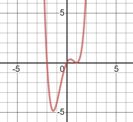
Curve Sketching
If a question consisted of just an equation and the directions that the student should draw a graph, how do you score it? How accurate does the graph need to be? Exactly what needs to be included?
An even bigger concern is what do you do if a student makes a small mistake, maybe just miscopies the equation? The problem may have become easier (say, an asymptote goes missing in the miscopied equation and if there is a point or two for dealing with asymptotes – what becomes of those points?) Is it fair to the student to lose points for something his small mistake made it unnecessary for him to consider? Or if the mistake makes the question so difficult it cannot be solved by hand, what happens then? Either way, the student knows what to do, yet cannot show that to the reader.
To overcome problems like these, the questions include several parts usually unrelated to each other, so that a mistake in one part does not make it impossible to earn any subsequent points. All the main ideas related to derivatives and graphing are tested somewhere on the exam, if not in the free-response section, then as a multiple-choice question.
(Where the parts are related, a wrong answer from one part, usually just a number, imported into the next part is considered correct for the second part and the reader then can determine if the student knows the concept and procedure for that part.)
Optimization
A big topic in derivative applications is optimization. Questions on optimization typically present a “real life” situation such as something must be built for the lowest cost or using the least material. The last question of this type was in 1982 (1982 AB 6, BC 3 same question). The question is 3.5 lines long and has no parts – just “find the cost of the least expensive tank.”
The problem here is the same as with curve sketching. The first thing the student must do is write the equation to be optimized. If the student does that incorrectly, there is no way to survive, and no way to grade the problem. While it is fair to not to award points for not writing the correct equation, it is not fair to deduct other points that the student could earn had he written the correct equation.
The main tool for optimizing is to find the extreme value of the function; that is tested on every exam. So here is a topic that you certainly may include the full question in you course, but the concepts will be tested in other ways on the exam.
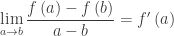
The epsilon-delta definition of limit
I think the reason that this topic is not tested is slightly different. If the function for which you are trying to “prove” the limit is linear, then  where m is the slope of the line – there is nothing to do beside memorize the formula. If the function is not linear, then the algebraic gymnastics necessary are too complicated and differ greatly depending on the function. You would be testing whether the student knew the appropriate “trick.”
Furthermore, in a multiple-choice question, the distractor that gives the smallest value of must be correct (even if a larger value is also correct).
Moreover, finding the epsilon-delta relationship is not what’s important about the definition of limit. Understanding how the existence of such a relationship say “gets closer to” or “approaches” in symbols and guarantees that the limit exists is important.
Volumes using the Shell Method
I have no idea why this topic is not included. It was before 1998. The only reason I can think of is that the method is so unlike anything else in calculus (except radial density), that it was eliminated for that reason.
This is a topic that students should know about. Consider showing it too them when you are doing volumes or after the exam. Their college teachers may like them to know it.
Integration by Parts on the AB exam
Integration by Parts is considered a second semester topic. Since AB is considered a one-semester course, Integration by Parts is tested on the BC exam, but not the AB exam. Even on the BC exam it is no longer covered in much depth: two- or more step integrals, the tabular method, and reduction formulas are not tested.
This is a topic that you can include in AB if you have time or after the exam or expand upon in a BC class.
Newton’s Method, Work, and other applications of integrals and derivatives
There are a great number of applications of integrals and derivatives. Some that were included on the exams previously are no longer listed. And that’s the answer right there: in fairness, you must tell students (and teachers) what applications to include and what will be tested. It is not fair to wing in some new application and expect nearly half a million students to be able to handle it.
Also, remember when looking through older exams, especially those from before 1998, that some of the topics are not on the current course description and will not be tested on the exams.
Solution of differential equations by methods other than separation of variables
Differential equations are a huge and important area of calculus. The beginning courses, AB and BC, try to give students a brief introduction to differential equations. The idea, I think, is like a survey course in English Literature or World History: there is no time to dig deeply, but the is an attempt to show the main parts of the subject.
While the choices are somewhat arbitrary, the College Board regularly consults with college and university mathematics departments about what to include and not include. The relatively minor changes in the new course description are evidence of this continuing collaboration. Any changes are usually announced two years in advance. (The recent addition of density problems unannounced, notwithstanding.) So, find a balance for yourself. Cover (or better yet, uncover) the ideas and concepts in the course description and if there if a topic you particularly like or think will help your students’ understanding of the calculus, by all means include it.
PS: Please scroll down and read Verge Cornelius’ great comment below.
Happy Holiday to everyone. There is no post scheduled for next week; I will resume in the new year. As always, I like to hear from you. If you have anything calculus-wise you would like me to write about, please let me know and I’ll see what I can come up with. You may email me at lnmcmullin@aol.com
.


 , so, substituting
  we have


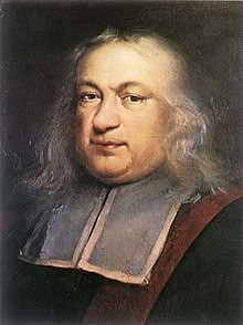
 – Fermat unknowingly is using the derivative! After which he set it equal to 0 and solved to find the
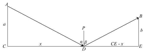
 and
and  are all perpendicular to
  the total distance is AD + DB. Therefore:
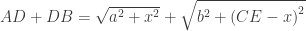


 and
and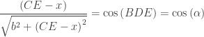
 QED.
QED.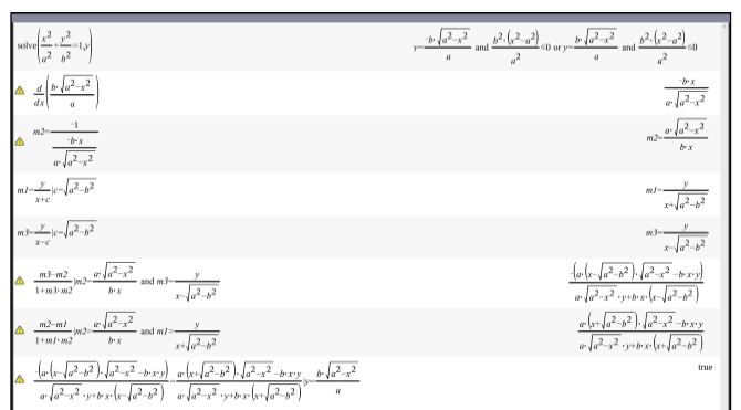
 with a > b > 0. Solving for y there are two equations, the second one is for the upper half that we will use below. The other for the lower half.
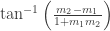
 and
and  .
. to avoid working with an undefined slope. The focus is at
  .
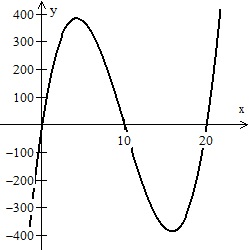
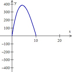
. . Why? Ignore the physical situation and determine the domain of the expression for the volume from a. Graph the function. Discuss.
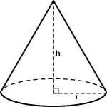
 , so
, so  and
and 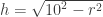 . The volume of the cone is


 ) gives

 . Then, solving for x gives
 and a height of
  . Its volume is
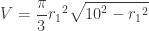
 . The computation and result will be the same. The result will be the same. The maximum occurs at
 . To graph there is no need to simplify the expression in x:
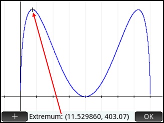


 . This isn’t really easier to differentiate and solve.
 and so the circumference of the base of the cone is
  and its radius is
 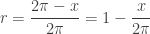 . The height, h of the cone is
 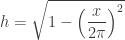 . See figure 4.
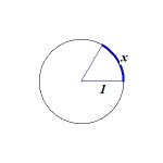

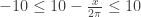
 . But if
  the piece you cut out will be larger than the original disk (and the expression under the radical will be negative). So our domain will be
  (the endpoints correspond to not cutting any sector or cutting away the entire disk. The graph is shown in Figure 6 with, alas, only one extreme value.
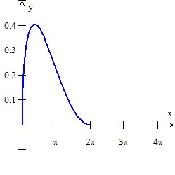
 and the maximums are at
  . A CAS will help with these calculations or just use a graphing calculator.)