2019 CED Unit 5 Analytical Applications of Differentiation

Unit 5 covers the application of derivatives to the analysis of functions and graphs. Reasoning and justification of results are also important themes in this unit. (CED – 2019 p. 92 – 107). These topics account for about 15 – 18% of questions on the AB exam and 8 – 11% of the BC questions.

Reasoning and writing justification of results are mentioned and stressed in the introduction to the topic (p. 93) and for most of the individual topics. See Learning Objective FUN-A.4 “Justify conclusions about the behavior of a function based on the behavior of its derivatives,” and likewise in FUN-1.C for the Extreme value theorem, and FUN-4.E for implicitly defined functions. Be sure to include writing justifications as you go through this topic. Use past free-response questions as exercises and also as guide as to what constitutes a good justification. Links in the margins of the CED are also helpful and give hints on writing justifications and what is required to earn credit. See the presentation Writing on the AP Calculus Exams and its handout

Topics 5.1

Topic 5.1 Using the Mean Value Theorem While not specifically named in the CED, Rolle’s Theorem is a lemma for the Mean Value Theorem (MVT). The MVT states that for a function that is continuous on the closed interval and differentiable over the corresponding open interval, there is at least one place in the open interval where the average rate of change equals the instantaneous rate of change (derivative). This is a very important existence theorem that is used to prove other important ideas in calculus. Students often confuse the average rate of change, the mean value, and the average value of a function – See What’s a Mean Old Average Anyway?

Topics 5.2 – 5.9

Topic 5.2 Extreme Value Theorem, Global Verses Local Extrema, and Critical Points An existence theorem for continuous functions on closed intervals

Topic 5.3 Determining Intervals on Which a Function is Increasing or Decreasing Using the first derivative to determine where a function is increasing and decreasing.

Topic 5.4 Using the First Derivative Test to Determine Relative (Local) Extrema Using the first derivative to determine local extreme values of a function

Topic 5.5 Using the Candidates’ Test to Determine Absolute (Global) Extrema The Candidates’ test can be used to find all extreme values of a function on a closed interval

Topic 5.6 Determining Concavity of Functions on Their Domains FUN-4.A.4 defines (at least for AP Calculus) When a function is concave up and down based on the behavior of the first derivative. (Some textbooks may use different equivalent definitions.) Points of inflection are also included under this topic.

Topic 5.7 Using the Second Derivative Test to Determine Extrema Using the Second Derivative Test to determine if a critical point is a maximum or minimum point. If a continuous function has only one critical point on an interval, then it is the absolute (global) maximum or minimum for the function on that interval.

Topic 5.8 Sketching Graphs of Functions and Their Derivatives. First and second derivatives give graphical and numerical information about a function and can be used to locate important points on the graph of the function.

Topic 5.9 Connecting a Function, Its First Derivative, and Its Second Derivative. First and second derivatives give graphical and numerical information about a function and can be used to locate important points on the graph of the function.

Topics 5.10 – 5.11

Optimization is important application of derivatives. Optimization problems as presented in most text books, begin with writing the model or equation that describes the situation to be optimized. This proves difficult for students, and is not “calculus” per se. Therefore, writing the equation has not be asked on AP exams in recent years (since 1983). Questions give the expression to be optimized and students do the “calculus” to find the maximum or minimum values. To save time, my suggestion is to not spend too much time writing the equations; rather concentrate on finding the extreme values.

Topic 5.10 Introduction to Optimization Problems 

Topic 5.11 Solving Optimization Problems

Topics 5.12

Topic 5.12 Exploring Behaviors of Implicit Relations Critical points of implicitly defined relations can be found using the technique of implicit differentiation. This is an AB and BC topic. For BC students the techniques are applied later to parametric and vector functions.


Timing

Topic 5.1 is important and may take more than one day. Topics 5.2 – 5.9 flow together and for graphing they are used together; after presenting topics 5.2 – 5.7 spend the time in topics 5.8 and 5.9 spiraling and connecting the previous topics. Topics 5.10 and 5.11 – see note above and spend minimum time here. Topic 5.12 may take 2 days.

The suggested time for Unit 5 is 15 – 16 classes for AB and 10 – 11 for BC of 40 – 50-minute class periods, this includes time for testing etc.

Finally, were I still teaching, I would teach this unit before Unit 4. The linear motion topic (in Unit 4) are a special case of the graphing ideas in Unit 5, so it seems reasonable to teach this unit first. See Motion Problems: Same thing, Different Context


Previous posts on these topics include:

Then There Is This – Existence Theorems

What’s a Mean Old Average Anyway

Did He, or Didn’t He?   History: how to find extreme values without calculus

Mean Value Theorem

Foreshadowing the MVT

Fermat’s Penultimate Theorem

Rolle’s theorem

The Mean Value Theorem I

The Mean Value Theorem II

Graphing

Concepts Related to Graphs

The Shapes of a Graph

Joining the Pieces of a Graph

Extreme Values

Extremes without Calculus

Concavity

Reading the Derivative’s Graph

Real “Real-life” Graph Reading

Far Out! An exploration

Open or Closed  Should intervals of increasing, decreasing, or concavity be open or closed?

Others

Lin McMullin’s Theorem and More Gold  The Golden Ratio in polynomials

Soda Cans  Optimization video

Optimization – Reflections   

Curves with Extrema?

Good Question 10 – The Cone Problem

Implicit Differentiation of Parametric Equations    BC Topic


Here are links to the full list of posts discussing the ten units in the 2019 Course and Exam Description.

2019 CED – Unit 1: Limits and Continuity

2019 CED – Unit 2: Differentiation: Definition and Fundamental Properties.

2019 CED – Unit 3: Differentiation: Composite , Implicit, and Inverse Functions

2019 CED – Unit 4 Contextual Applications of the Derivative  Consider teaching Unit 5 before Unit 4

2019 – CED Unit 5 Analytical Applications of Differentiation  Consider teaching Unit 5 before Unit 4

2019 – CED Unit 6 Integration and Accumulation of Change

2019 – CED Unit 7 Differential Equations  Consider teaching after Unit 8

2019 – CED Unit 8 Applications of Integration   Consider teaching after Unit 6, before Unit 7

2019 – CED Unit 9 Parametric Equations, Polar Coordinates, and Vector-Values Functions 

2019 CED Unit 10 Infinite Sequences and Series


Advertisement

Then there is this – Existence Theorems

Existence Theorems

An existence theorem is a theorem that says, if the hypotheses are met, that something, usually a number, must exist.

For example, the Mean Value Theorem is an existence theorem: If a function f is defined on the closed interval [a, b] and differentiable on the open interval (a, b), then there exists a number c in the open interval (a, b) such that \displaystyle {f}'\left( c \right)\left( {b-a} \right)=f\left( b \right)-f\left( a \right).

The phrase “there exists” can also mean “there is” and “there is at least one.” In fact, it is a good idea when seeing an existence theorem to reword it using each of these other phrases. “There is at least one” reminds you that there may be more than one number that satisfies the condition. The mathematical symbol for these phrases is an upper-case E written backwards: \displaystyle \exists .

Textbooks, after presenting an existence theorem, usually follow-up with some exercises asking students to find the value for a given function on a given interval: “Find the value of c guaranteed by the Mean Value Theorem for the function … on the interval ….” These exercises may help students remember the formula involved but are not very useful otherwise.

The important thing about most existence theorems is that the number exists, not what the number is. To illustrate this, let’s consider the Fundamental Theorem of Calculus. After partitioning the interval [a, b] into subintervals at various values, xi, we consider the limit of the sum

\displaystyle \underset{{n\to \infty }}{\mathop{{\lim }}}\,\sum\limits_{{n=1}}^{n}{{\left( {f\left( {{{x}_{i}}} \right)-f\left( {{{x}_{{i-1}}}} \right)} \right)}}.

Write out a few terms and you will see that is a telescoping series and its limit is \displaystyle f\left( b \right)-f\left( a \right).

The expression \displaystyle {f\left( {{{x}_{i}}} \right)-f\left( {{{x}_{{i-1}}}} \right)} resembles the right side of the Mean Value Theorem above. Since all the conditions are met, the MVT tells us that in each subinterval \displaystyle [{{x}_{{i-1}}},{{x}_{i}}] there exists a number, call it ci , such that

\displaystyle {f}'\left( {{{c}_{i}}} \right)\left( {{{x}_{i}}-{{x}_{{i-1}}}} \right)=f\left( {{{x}_{i}}} \right)-f\left( {{{x}_{{i-1}}}} \right) and therefore

\displaystyle \underset{{n\to \infty }}{\mathop{{\lim }}}\,\sum\limits_{{n=1}}^{n}{{\left( {f\left( {{{x}_{i}}} \right)-f\left( {{{x}_{{i-1}}}} \right)} \right)}}=\underset{{n\to \infty }}{\mathop{{\lim }}}\,\sum\limits_{{n=1}}^{n}{{{f}'\left( {{{c}_{i}}} \right)\left( {{{x}_{i}}-{{x}_{{i-1}}}} \right)}}=f\left( b \right)-f\left( a \right)

No one is concerned what these ci are, just that there are such numbers, that they exist. (The second limit above is then defined as the definite integral so \displaystyle \underset{{n\to \infty }}{\mathop{{\lim }}}\,\sum\limits_{{n=1}}^{n}{{{f}'\left( {{{c}_{i}}} \right)\left( {{{x}_{i}}-{{x}_{{i-1}}}} \right)}}=\int_{a}^{b}{{{f}'\left( x \right)dx=}}f\left( b \right)-f\left( a \right) – The Fundamental Theorem of Calculus.)

Other important existence theorems in calculus

The Intermediate Value Theorem

If f is continuous on the interval [a, b] and M is any number between f(a) and f(b), then there exists a number c in the open interval (a, b) such that f(c) = M.

If f is continuous on an interval and f changes sign in the interval, then there must be at least one number c in the interval such that f(c) = 0

Extreme Value Theorem

If f is continuous on the closed interval [a, b], then there exists a number c in [a, b] such that \displaystyle f\left( c \right)\ge f\left( x \right) for all x in the interval. Every function continuous on a closed interval has (i.e. there exists) a maximum value in the interval.

If f is continuous on the closed interval [a, b], then there exists a number c in [a, b] such that \displaystyle f\left( c \right)\le f\left( x \right) for all x in the interval. Every function continuous on a closed interval has (i.e. there exists) a minimum value in the interval.

Critical Points

If f is differentiable on a closed interval and \displaystyle {f}'\left( x \right) changes sign in the interval, then there exists a critical point in the interval.

Rolle’s theorem

If a function f is defined on the closed interval [a, b] and differentiable on the open interval (a, b) and f(a) = f(b), then there must exist a number c in the open interval (a, b) such that \displaystyle {f}'\left( c \right)=0.

MVT – other forms

If I drive a car continuously for 150 miles in three hours, then there is a time when my speed was exactly 50 mph.

If a function f is defined on the closed interval [a, b] and differentiable on the open interval (a, b), then there is a point on the graph of f where the tangent line is parallel to the segment between the endpoints.

Taylor’s Theorem

If f is a function with derivatives through order n + 1 on an interval I containing a, then, for each x in I , there exists a number c between x and a such that

\displaystyle f\left( x \right)=\sum\limits_{k=0}^{n}{\frac{{{f}^{\left( k \right)}}\left( a \right)}{k!}{{\left( x-a \right)}^{k}}}+\frac{{{f}^{\left( n+1 \right)}}\left( c \right)}{\left( n+1 \right)!}{{\left( x-a \right)}^{n+1}}

The number \displaystyle R=\frac{{{f}^{\left( n+1 \right)}}\left( c \right)}{\left( n+1 \right)!}{{\left( x-a \right)}^{n+1}} is called the remainder. The equation above says that if you can find the correct c the function is exactly equal to Tn(x) + R. Notice the form of the remainder is the same as the other terms, except it is evaluated at the mysterious c. The trouble is we almost never can find the c without knowing the exact value of f(x), but; if we knew that, there would be no need to approximate. However, often without knowing the exact values of c, we can still approximate the value of the remainder and thereby, know how close the polynomial Tn(x) approximates the value of f(x) for values in x in the interval, i. See Error Bounds and the Lagrange error bound.

Cogito, ergo sum

And finally, we have Descartes’ famous “theorem” Cogito, ergo sum (in Latin) or the original French, Je pense, donc je suis, translated as “I think, therefore I am” proving his own existence.


The Mean Value Theorem

Another application of the derivative is the Mean Value Theorem (MVT). This theorem is very important. One of its most important uses is in proving the Fundamental Theorem of Calculus (FTC), which comes a little later in the year. Here are some previous post on the MVT:

Fermat’s Penultimate Theorem   A lemma for Rolle’s Theorem: Any function extreme value(s) on an open interval must occur where the derivative is zero or undefined.

Rolle’s Theorem   A lemma for the MVT: On an interval if a function is continuous on a closed interval [a, b] and differentiable on the open interval (a, b) and f(a) = f(b), there must exist a number in the open interval (a, b) where ‘(c) = 0.

Mean Value Theorem I   Proof

Mean Value Theorem II   Graphical Considerations

Darboux’s Theorem   The Intermediate Value Theorem for derivatives.

Mean Tables


Darboux’s Theorem

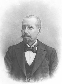
Jean Gaston Darboux 1842 - 1917

Jean Gaston Darboux
1842 – 1917

Jean Gaston Darboux was a French mathematician who lived from 1842 to 1917. Of his several important theorems the one we will consider says that the derivative of a function has the Intermediate Value Theorem property – that is, the derivative takes on all the values between the values of the derivative at the endpoints of the interval under consideration.

Darboux’s Theorem is easy to understand and prove but is not usually included in a first-year calculus course (and is not included on the AP exams). Its use is in the more detailed study of functions in a real analysis course.

You may want to use this as an enrichment topic in your calculus course, or a topic for a little deeper investigation. The ideas here are certainly within the range of what first-year calculus students should be able to follow. They relate closely to the Mean Value Theorem (MVT). I will suggest some ideas (in blue) to consider along the way.

More precisely Darboux’s theorem says that

If f is differentiable on the closed interval [a, b] and r is any number between f ’ (a) and f ’ (b), then there exists a number c in the open interval (a, b) such that ‘ (c) = r. 

Differentiable on a closed interval?

Most theorems in beginning calculus require only that the function be differentiable on an open interval. Here, obviously, we need a closed interval so that there will be values of the derivative for r to be between.

The limit definition of derivative requires a regular two-sided limit to exist; at the endpoint of an interval there is only one side. For most theorems this is enough. Here the definition of derivative must be extended to allow one-sided limits as x approaches the endpoint values from inside the interval. Also note that  if a function is differentiable on (a, b), then it is differentiable on any closed sub-interval of (a, b) that does not include a or b.

Geometric proof [1]

Consider the diagram below, which shows a function in blue. At each endpoint draw a line with the slope of r. Notice that these two lines have a slope less than that of the function at the left end and greater than the slope at the right end. At least one of these lines must intersect the function at an interior point of the interval.  Before reading on, see if you and your students can complete the proof from here. (Hint: What theorem does the top half of the figure remind you of?)

DarbouxOn the interval between the intersection point and the end point we can apply the Mean Value Theorem and determine the value of c where the tangent line will be parallel to the line through the endpoint. At this point ‘(c) = r. Q.E.D.

Analytic Proof [2]

Consider the function h\left( x \right)=f\left( x \right)-(f(b)+r(x-b)). Since f(x) is differentiable, it is continuous; \displaystyle f(b)+r(x-a) is also continuous and differentiable. Therefore, h(x) is continuous and differentiable on [a, b]. By the Extreme Value Theorem, there must be a point, x = c, in the open interval (a, b) where h(x) has an extreme value. At this point h’ (c) = 0.

Before reading on see if you can complete the proof from here.

\displaystyle h(x)=f(x)-(f(b)+r(x-a))

\displaystyle {h}'(x)={f}'(x)-r

\displaystyle {h}'(c)={f}'(c)-r=0

\displaystyle {f}'\left( c \right)=r

Q.E.D.

Exercise: Compare and contrast the two proofs.

  1. In the geometric proof, what does \displaystyle y=f(b)+r(x-a) represent? Where does it show up in the diagram?
  2. How do both proofs relate to the Mean Value Theorem (or Rolle’s Theorem).

The function \displaystyle h(x)=f(x)-(f(b)+r(x-a)) represents the vertical distance from f(x) to \displaystyle f(b)+r(x-a). In the diagram, this is a vertical segment connecting f(x) to  \displaystyle y=f(b)+r(x-a).This expression may be positive, negative, or zero. In the diagram, at the point(s) where the line through the right endpoint intersects the curve and at the endpoint h(x) = 0. Therefore, h(x) meets the hypotheses of Rolle’s Theorem (and the MVT), and the result follows.

The line through the right endpoint will have equation the y=f(b)+r(x-b) This makes h\left( x \right)=f\left( x \right)-\left( f(b)+r(x-b) \right). When differentiated and the result will be {f}'\left( x \right)-r the same expression as in the analytic proof.

Also, you may move this line upwards parallel to its original position and eventually it will be tangent to the graph of the function. (See my posts on MVT 1 and especially MVT 2).

Exercise:

Consider the function f(x) = sin(x)

  1. On the interval [1,3] what values of the derivative of f are guaranteed by Darboux’s Theorem? .
  2. Does Darboux’s theorem guarantee any value on the interval [0,2\pi ]? Why or why not?

Answers:

  1. f ‘(x) = cos(x). f ‘ (1) = 0.54030 and f ‘ (3) = -0.98999. So the guaranteed values are from -0.98999 to 0.54030.
  2. No. f ‘ (x) = 1 at both endpoints, so there are no values between one and one.

Another interesting aspect of Darboux’s Theorem is that there is no requirement that the derivative ‘(x) be continuous!

A common example of such a function is

\displaystyle f\left( x \right)=\left\{ \begin{matrix} {{x}^{2}}\sin \left( \frac{1}{x} \right) & x\ne 0 \\ 0 & x=0 \\ \end{matrix} \right.

With \displaystyle {f}'\left( x \right)=-\cos \left( \tfrac{1}{x} \right)+2x\sin \left( \tfrac{1}{x} \right),\,\,x\ne 0.

This function (which has appeared on the AP exams) is differentiable (and therefore continuous).There is an oscillating discontinuity at the origin. The derivative is not continuous at the origin.  Yet, every interval containing the origin as an interior point meets the conditions of Darboux’s Theorem, so the derivative while not continuous has the intermediate value property.

AP exam question 1999 AB3/BC3 part c:

Finally, what inspired this post was a recent discussion on the AP Calculus Community bulletin board about the AP exam question 1999 AB3/BC3 part c. This question gave a table of values for the rate, R, at which water was flowing out of a pipe as a differentiable function of time t. The question asked if there was a time when R’ (t) = 0. It was expected that students would use Rolle’s Theorem or the MVT. There was a discussion about using Darboux’s theorem or saying something like the derivative increased (or was positive), then decreased (was negative) so somewhere the derivative must be zero (implying that derivative had the intermediate value property). Luckily, no one tried this approach, so it was a moot point.

Take a look at the problem with your students and see if you can use Darboux’s theorem. Be sure the hypotheses are met.

Answer (try it yourself before reading on):

The function is not differentiable at the endpoints. But consider an interval like [0,3]. Using the given values in the table, by the MVT there is a time t = c where R‘(c) = 0.8/3 > 0, and there is a time t = d on the interval [21, 24] where R‘(d) = -0.6/3 < 0. The function is differentiable on the closed interval [c, d] so by Darboux’s Theorem there must exist a time when R’(t) = 0. Admittedly, this is a bit of overkill.

References:

  1. After Nitecki, Zbigniew H. Calculus Deconstructed A Second Course in First-Year Calculus, ©2009, The Mathematical Association of America, ISBN 978-0-883835-756-4, p. 221-222.
  2. After Dunham, William The Calculus Gallery Masterpieces from Newton to Lebesque, © 2005, Princeton University Press, ISBN 978-0-691-09565-3, p. 156.

Both these book are good reference books.

Updated: August 20, 2014, and October 4, 2017

The Mean Value Theorem II

The Rule of Four suggests that mathematics be studied from the analytical, graphical, numerical, and verbal points of view. Proof can only be done analytically – using symbols and equations. Graphs, numbers, and words aid in that, but do not by themselves prove anything.

On the other hand, numbers and especially graphs can make many of the theorems much more understandable and often can convince one of the truth of a theorem far better than the actual proof.

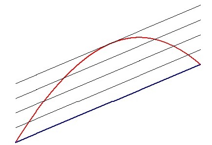
The Mean Value Theorem, MVT, is a good example; it can be demonstrated with a lot less trouble. See the figure above. Picture the blue line connecting the endpoints of the interval (the secant line) moving up, parallel to its original position. See the figure above. As this line moves up it intersects the graph twice, until eventually, just before it does not intersect at all, it comes to a place where it intersects exactly one. At this point it is tangent to the original graph. Since it is tangent, the slope of the line is the same as the derivative, {f}'\left( c \right), at that point.

So, the derivative is equal to the slope of the line between the endpoints. The MVT says that if its hypotheses are true, then there must be a place where the slope of the tangent line is parallel to the slope of the secant line.
But wait, there is more: at that point the instantaneous rate of change of the function is equal to the average rate of change over the interval.

This shows a real strength of looking at the graph.

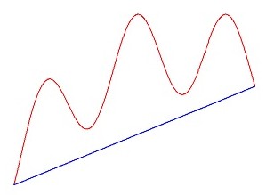
But it is only one of many possible graphs. The graph could look like this figure:

Here there are several places (5 to be exact) where the tangent line is parallel to the secant line; there could be several on one side, or several on both sides. But this is not a problem; this does not contradict the MVT, which says there is at least one.

Yet another way to show the MVT is this. Near the left end of the first graph above the slope of the tangent to the graph (the derivative) is larger than the slope of the secant line; near the right end the slope of the tangent is less than the slope of the secant. So somewhere in between, by the Intermediate Value Theorem, the slope of the tangent must equal the slope of the secant. (For the purists out there, this is from Darboux’s theorem, and requires a slightly stronger hypothesis, namely that the one-sided derivatives at a and b exist.)

Rolle’s theorem can be demonstrated with either of these approaches as well. Rolle’s Theorem is really a special case of the MVT where the slope of the secant line is zero.

In conclusion, I think that this sequence of theorems is a good place to do a little proving of theorems. On the other hand you can easily show the results other ways. In fact, the method at the beginning of this post should be shown anyway in order to give students a good picture (no pun intended) of the MVT. It will help them remember what it is all about.

Rolle’s Theorem

Rolle’s theorem says that if a function is continuous on a closed interval [a, b], differentiable on the open interval (a, b) and if f (a) = f (b), then there exists a number c in the open interval (a, b) such that {f}'\left( c \right)=0.  (“There exists a number” means that there is at least one such number; there may be more than one.)

The proof has two cases:

Case I: The function is constant (all of the values of the function are the same as f (a) and f (b)). The derivative of a constant is zero so any (every, all) value(s) in the open interval qualifies as c.

Case II: If the function is not constant then it must have a maximum or minimum in the open interval (a, b) by the Extreme Value Theorem. So, by Fermat’s theorem (see this post) the derivative at that point must be zero.

So, Fermat’s theorem makes Rolle’s theorem a piece of cake.

A lemma is a theorem whose result is used in the next theorem and makes it easier to prove. So Fermat’s theorem is a lemma for Rolle’s theorem.

On the other hand, a corollary is a theorem is a result (theorem) that follows easily from the previous theorem. So, Rolle’s theorem could also be called a corollary of Fremat’s theorem.

Rolle’s theorem makes a major appearance in the MVT and then more or less disappears from the stage. When you find critical number or critical points you are using Fermat’s theorem.

I like this proof because it’s so simple. It really just comes immediately from Fermat’s theorem.

The next post: The Mean Value Theorem.