Determining the Indeterminate

Posted on September 24, 2015 by Lin McMullin

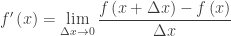
When determining the limit of an expression the first step is to substitute the value the independent variable approaches into the expression. If a real number results, you are all set; that number is the limit.

When you do not get a real number often expression is one of the several indeterminate forms listed below:

Indeterminate Forms:

$\displaystyle \frac{0}{0},\quad \quad \frac{\pm \infty }{\pm \infty },\quad \quad 0\cdot \infty ,\quad \quad \infty -\infty ,\quad \quad {{0}^{0}},\quad \quad {{1}^{\infty }},\quad \quad {{\infty }^{0}}$

They are called indeterminate forms because by doing some algebraic manipulation to simplify (or sometimes complicate) the expression its value can be determined. The calculus technique called L’Hôpital’s Rule may be used in some situations.

Part of the reason they are called indeterminate forms is that different expressions with the same indeterminate form may result in different values.

Before continuing with the discussion of indeterminate forms, I should point out that there are also determinate forms: expressions similar to those above that always result in the same value.

Determinate Forms and the values they approach:

$\displaystyle \frac{1}{\pm \infty }\to 0,\quad \infty +\infty \to \infty ,\quad \infty \cdot \infty \to \infty ,\quad {{0}^{\infty }}\to 0,\quad \frac{1}{{{0}^{\infty }}}={{0}^{-\infty }}\to \infty$

Returning to indeterminate forms, textbooks contain examples and exercises that illustrate how to evaluate the indeterminate forms. Here are two examples illustrating a few of the techniques that can be used to evaluate them.

Example 1: $\displaystyle \underset{x\to \infty }{\mathop{\lim }}\,{{\left( 1+\frac{1}{x} \right)}^{x}}=?$ .This is an example of the indeterminate form ${{1}^{\infty }}$ . With exponents, logarithms may often be used to find the value.

The limit is now of the indeterminate form $\frac{0}{0}$ , so L’Hôpital’s Rule may be used. Continuing

$\displaystyle \ln \left( ? \right)=\underset{x\to \infty }{\mathop{\lim }}\,\left( x\ln \left( 1+\frac{1}{x} \right) \right)=\underset{x\to \infty }{\mathop{\lim }}\,\frac{\ln \left( 1+\frac{1}{x} \right)}{\frac{1}{x}}=\underset{x\to \infty }{\mathop{\lim }}\,\frac{\left( \frac{1}{1+\frac{1}{x}} \right)\left( -{{x}^{-2}} \right)}{-{{x}^{-2}}}=\underset{x\to \infty }{\mathop{\lim }}\,\left( \frac{1}{1+\frac{1}{x}} \right)=1$

So then ln(?) = 1 and ? = e¹ = e and therefore $\displaystyle \underset{x\to \infty }{\mathop{\lim }}\,{{\left( 1+\frac{1}{x} \right)}^{x}}=e$

Example 2: $\displaystyle \underset{x\to 0}{\mathop{\lim }}\,\left( \frac{\sin \left( x+\frac{\pi }{6} \right)}{x}-\frac{\sin \left( \frac{\pi }{6} \right)}{x} \right)$ is an example of the indeterminate form $\infty -\infty$ .

Write the expression with a common denominator:

$\displaystyle \underset{x\to 0}{\mathop{\lim }}\,\left( \frac{\sin \left( x+\frac{\pi }{6} \right)}{x}-\frac{\sin \left( \frac{\pi }{6} \right)}{x} \right)=\underset{x\to 0}{\mathop{\lim }}\,\left( \frac{\sin \left( \frac{\pi }{6}+x \right)-\sin \left( \frac{\pi }{6} \right)}{x} \right)=\cos \left( \frac{\pi }{6} \right)=\frac{\sqrt{3}}{2}$

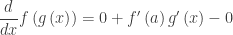
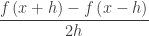
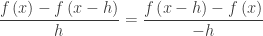
The second limit above is the definition of the derivative of $\sin \left( \frac{\pi }{6} \right)$ . (L’Hôpital’s Rule may also be used with the second limit above.)

In fact, the definition of the derivative of all (any, every) functions, $\displaystyle {f}'\left( a \right)=\underset{h\to 0}{\mathop{\lim }}\,\frac{f\left( a+h \right)-f\left( a \right)}{h}$ , gives indeterminate expressions of the form $\frac{0}{0}$ .

Foreshadowing the FTC

Posted on December 15, 2014 by Lin McMullin

This is an example to help prepare students to tackle the Fundamental Theorem of Calculus (FTC). Use it after the lesson on Riemann sums and the definition of the definite integral, but before the FTC derivation.

Consider the area, A, between the graph of $f\left( x \right)=\cos \left( x \right)$ and the x-axis on the interval $\left[ 0,\tfrac{\pi }{2} \right]$ . Set up a Riemann sum using the general partition:

$0={{x}_{0}}<{{x}_{1}}<{{x}_{2}}<{{x}_{3}}<\cdots <{{x}_{n-2}}<{{x}_{n-1}}<{{x}_{n}}=\tfrac{\pi }{2}$

$\displaystyle A=\int_{0}^{{\scriptstyle{}^{\pi }\!\!\diagup\!\!{}_{2}\;}}{\cos \left( x \right)dx}=\underset{\Delta x\to 0}{\mathop{\lim }}\,\sum\limits_{i=1}^{n}{\cos \left( {{c}_{i}} \right)\left( {{x}_{i}}-{{x}_{i-1}} \right)}$

Since we can choose the value of ${{c}_{i}}$ any way we want, let’s take the same intervals and use ${{c}_{i}}$ the number guaranteed by the Mean Value Theorem for the function $F\left( x \right)=\sin \left( x \right)$ on the each sub-interval interval. That is, on each sub-interval at $x={{c}_{i}}$

$\left. \frac{d}{dx}\sin \left( x \right) \right|_{x={{c}_{i}}}^{{}}=\cos \left( {{c}_{i}} \right)=\frac{\sin \left( {{x}_{i}} \right)-\sin \left( {{x}_{i-1}} \right)}{\left( {{x}_{i}}-{{x}_{i-1}} \right)}$

Then, substituting into the Riemann sum above

$\displaystyle A=\underset{\Delta x\to 0}{\mathop{\lim }}\,\sum\limits_{i=1}^{n}{\cos \left( {{c}_{i}} \right)\left( {{x}_{i}}-{{x}_{i-1}} \right)}=\underset{\Delta x\to 0}{\mathop{\lim }}\,\sum\limits_{i=1}^{n}{\frac{\sin \left( {{x}_{i}} \right)-\sin \left( {{x}_{i-1}} \right)}{\left( {{x}_{i}}-{{x}_{i-1}} \right)}\left( {{x}_{i}}-{{x}_{i-1}} \right)}$

$\displaystyle A=\underset{\Delta x\to 0}{\mathop{\lim }}\,\sum\limits_{i=1}^{n}{\left( \sin \left( {{x}_{i}} \right)-\sin \left( {{x}_{i-1}} \right) \right)}$

Now writing out the terms we have a telescoping series:

$\displaystyle A=\left( \sin \left( {{x}_{1}} \right)-\sin \left( {{x}_{0}} \right) \right)+\left( \sin \left( {{x}_{2}} \right)-\sin \left( {{x}_{1}} \right) \right)+\left( \sin \left( {{x}_{3}} \right)-\sin \left( {{x}_{2}} \right) \right)+$

$\displaystyle \cdots +\left( \sin \left( {{x}_{n-1}} \right)-\sin \left( {{x}_{n-2}} \right) \right)+\left( \sin \left( {{x}_{n}} \right)-\sin \left( {{x}_{n-1}} \right) \right)$

$\displaystyle A=\sin \left( {{x}_{n}} \right)-\sin \left( {{x}_{0}} \right)$

$\displaystyle A=\sin \left( \tfrac{\pi }{2} \right)-\sin \left( 0 \right)=1$

As you can see, this is really just the derivation of the FTC applied to a particular function. Now the students should have a better idea of what’s going on when you solve the problem in general, i.e. when you prove the FTC.

Power Rule Implies Chain Rule

Posted on September 20, 2014 by Lin McMullin

Having developed the Product Rule $d\left( uv \right)=u{v}'+{u}'v$ and the Power Rule $\frac{d}{dx}{{x}^{n}}=n{{x}^{n-1}}$ for derivatives in your class, you can explore similar rules for the product of more than two functions and suddenly the Chain Rule will appear.

For three functions use the associative property of multiplication with the rule above:

$d\left( uvw \right)=d\left( \left( uv \right)w \right)=u\cdot v\cdot dw+w\cdot d(uv)=u\cdot v\cdot dw+w\left( udv+vdu \right)$

So expanding with a slight change in notation:

$d\left( uvw \right)=uv{w}'+u{v}'w+u'vw$

For four factors there is a similar result:

$d\left( uvwz \right)=uvw{z}'+uv{w}'z+u{v}'wz+{u}'vwz$

Exercise: Let ${{f}_{i}}$ for $i=1,2,3,...,n$ be functions. Write a general formula for the derivative of the product ${{f}_{1}}{{f}_{2}}{{f}_{3}}\cdots {{f}_{n}}$ as above and in sigma notation

Answers

$d\left( {{f}_{1}}{{f}_{2}}{{f}_{3}}\cdots {{f}_{n}} \right)={{f}_{1}}{{f}_{2}}{{f}_{3}}\cdots {{{f}'}_{n}}+{{f}_{1}}{{f}_{2}}{{{f}'}_{3}}\cdots {{f}_{n}}+{{f}_{1}}{{{f}'}_{2}}{{f}_{3}}\cdots {{f}_{n}}+\cdots +{{{f}'}_{1}}{{f}_{2}}{{f}_{3}}\cdots {{f}_{n}}$

$\displaystyle d\left( {{f}_{1}}{{f}_{2}}{{f}_{3}}\cdots {{f}_{n}} \right)=\sum\limits_{i=1}^{n}{\frac{{{f}_{1}}{{f}_{2}}{{f}_{3}}\cdots {{f}_{n}}}{{{f}_{i}}}{{{{f}'}}_{i}}}$

This idea may now be used to see the Chain Rule appear. Students may guess that $d{{\left( f \right)}^{4}}=4{{\left( f \right)}^{3}}$ , but wait there is more to it.

Write ${{\left( f \right)}^{4}}=f\cdot f\cdot f\cdot f\text{ }$ . Then from above

$d{{\left( f \right)}^{4}}=d\left( f\cdot f\cdot f\cdot f\text{ } \right)=f\cdot f\cdot f\cdot {f}'+f\cdot f\cdot {f}'\cdot f+f\cdot {f}'\cdot f\cdot f+{f}'\cdot f\cdot f\cdot f$

$d{{\left( f \right)}^{4}}=4{{\left( f \right)}^{3}}{f}'\text{ }$

Looks just like the power rule, but there’s that “extra” ${f}'$ . Now you are ready to explain about the Chain Rule in the next class.

The Mean Value Theorem II

Posted on October 1, 2012 by Lin McMullin

The Rule of Four suggests that mathematics be studied from the analytical, graphical, numerical, and verbal points of view. Proof can only be done analytically – using symbols and equations. Graphs, numbers, and words aid in that, but do not by themselves prove anything.

On the other hand, numbers and especially graphs can make many of the theorems much more understandable and often can convince one of the truth of a theorem far better than the actual proof.

The Mean Value Theorem, MVT, is a good example; it can be demonstrated with a lot less trouble. See the figure above. Picture the blue line connecting the endpoints of the interval (the secant line) moving up, parallel to its original position. See the figure above. As this line moves up it intersects the graph twice, until eventually, just before it does not intersect at all, it comes to a place where it intersects exactly one. At this point it is tangent to the original graph. Since it is tangent, the slope of the line is the same as the derivative, ${f}'\left( c \right)$ , at that point.

So, the derivative is equal to the slope of the line between the endpoints. The MVT says that if its hypotheses are true, then there must be a place where the slope of the tangent line is parallel to the slope of the secant line.
But wait, there is more: at that point the instantaneous rate of change of the function is equal to the average rate of change over the interval.

This shows a real strength of looking at the graph.

But it is only one of many possible graphs. The graph could look like this figure:

Here there are several places (5 to be exact) where the tangent line is parallel to the secant line; there could be several on one side, or several on both sides. But this is not a problem; this does not contradict the MVT, which says there is at least one.

Yet another way to show the MVT is this. Near the left end of the first graph above the slope of the tangent to the graph (the derivative) is larger than the slope of the secant line; near the right end the slope of the tangent is less than the slope of the secant. So somewhere in between, by the Intermediate Value Theorem, the slope of the tangent must equal the slope of the secant. (For the purists out there, this is from Darboux’s theorem, and requires a slightly stronger hypothesis, namely that the one-sided derivatives at a and b exist.)

Rolle’s theorem can be demonstrated with either of these approaches as well. Rolle’s Theorem is really a special case of the MVT where the slope of the secant line is zero.

In conclusion, I think that this sequence of theorems is a good place to do a little proving of theorems. On the other hand you can easily show the results other ways. In fact, the method at the beginning of this post should be shown anyway in order to give students a good picture (no pun intended) of the MVT. It will help them remember what it is all about.

The Chain Rule

Posted on September 21, 2012 by Lin McMullin

Except for the simplest functions, a procedure known as the Chain Rule is very helpful and often necessary to find derivatives. You can start with an example such as finding the derivative of ${{\left( 2x+7 \right)}^{2}}$ . Most students will expand the binomial to get $4{{x}^{2}}+28x+49$ and differentiate the result to get $8x+28$ . They will try the same approach with ${{\left( 2x+7 \right)}^{3}}$ and then you can hit them with ${{\left( 2x+7 \right)}^{53}}$ . They will see the need for a short cut at once. What to do?

The explanation runs like this. Let $u\left( x \right)={{x}^{53}}$ and let $v\left( x \right)=2x+7$ . Then our original expression becomes 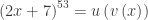${{\left( 2x+7 \right)}^{53}}=u\left( v\left( x \right) \right)$ a composition of functions. The Chain Rule is used for differentiating compositions. Students must get good at recognizing compositions. The differentiation is done from the outside, working inward. It is done in the exact opposite order than the procedure for evaluating expression. To evaluate the expression above you (1) evaluate the expression inside the parentheses and the (2) raise that result to the 53 power. To differentiate you (1) use the power rule to differentiate the 53 power of whatever is inside, this gives $53{{\left( 2x+7 \right)}^{52}}$ , the (2) differentiate the $\left( 2x+7 \right)$ which give 2 and multiply the results: $53{{\left( 2x+{{7}^{52}} \right)}^{52}}(2)=106{{\left( 2x+7 \right)}^{52}}$ . Symbolically, this looks like ${u}'\left( v\left( x \right) \right){v}'\left( x \right)$ or ${f}'\left( g\left( x \right) \right){g}'\left( x \right)$ . This can be extended to compositions of more than two functions:

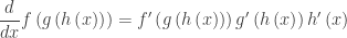
$\displaystyle \frac{d}{dx}f\left( g\left( h\left( x \right) \right) \right)={f}'\left( g\left( h\left( x \right) \right) \right){g}'\left( h\left( x \right) \right){h}'\left( x \right)$

The cartoon below is from Courtney Gibbons’ great collection of math cartoons (http://brownsharpie.courtneygibbons.org/) may help you kids remember this:

I have been looking for a way to illustrate the Chain Rule graphically, but to no avail. The closest I could come up with is this: Consider $f\left( x \right)=\sin \left( 3x \right)$ . This function takes on all the values of $y=\sin \left( x \right)$ in order in one-third the time. (That is its period is one-third of the period of $y=\sin \left( x \right)$ . Since this is true, it must go through the values three times as fast; thus, its derivative (it’s rate of change) must be three times the derivative of the sine: ${f}'\left( x \right)=3\cos \left( 3x \right)$ .

The students will need some practice on using the Chain Rule. I suggest a number of simple (single compositions) first and then a few longer ones and maybe one or two “monsters” just for fun once they get the idea.

The Chain Rule doesn’t end with just being able to differentiate complicated expressions; it will also form the basis for implicit differentiation, finding the derivative of a function’s inverse and Related Rate problems among others things.

Finally, here is a way to develop the Chain Rule which is probably different and a little more intuitive from what you will find in your textbook. (After a suggestion by Paul Zorn on the AP Calculus EDG October 14, 2002)

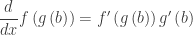
Let f be a function differentiable at $x=a$ , and let g be a function that is differentiable at $x=b$ and such that $g\left( b \right)=a$ . Then, near $x=a$ we can use the local linear approximation of f and g to find $\frac{d}{dx}f\left( g\left( b \right) \right)$ :

$f\left( x \right)\approx f\left( a \right)+{f}'\left( a \right)\left( x-a \right)$

$f\left( g\left( x \right) \right)\approx f\left( a \right)+{f}'\left( a \right)\left( g\left( x \right)-a \right)=f\left( a \right)+{f}'\left( a \right)g\left( x \right)-a {f}'\left( a \right)$

$\displaystyle \frac{d}{dx}f\left( g\left( x \right) \right)=0+{f}'\left( a \right){g}'\left( x \right)-0$

$\displaystyle\frac{d}{dx}f\left( g\left( b \right) \right)={f}'\left( g\left( b \right) \right){g}'\left( b \right)$

Difference Quotients II

Posted on September 12, 2012 by Lin McMullin

The Symmetric Difference Quotient

In the last post we defined the Forward Difference Quotient (FDQ) and the Backward Difference Quotient (BDQ). The average of the FDQ and the BDQ is called the Symmetric Difference Quotient (SDQ):

$\displaystyle \frac{f\left( x+h \right)-f\left( x-h \right)}{2h}$

You may be forgiven if you think this might be a better expression to use to find the derivative. It has its advantages. In fact, this is the expression used in many calculators to compute the numerical value of the derivative at a point; in calculators it is called nDeriv. Usually, it works pretty well. But if you try to find the derivative of the absolute value of x at x = 0 it will tell you the derivative is 0, which is wrong. The absolute value function is not locally linear at the origin and has no derivative there.

What went wrong? Read the expression above. The numerator is the difference of the function values at the same distance, h, on both sides of x. Since, for the absolute value function with x = 0, these values are the same, their difference is 0. The SDQ never looks at x = 0 and doesn’t realize there is no derivative there. Thus, the limit of the SDQ is not the derivative.

This problem does not occur with the definition of derivative, since for that limit to exist the limits as h approaches zero from both sides must be equal. For the absolute value function the limit from the left is –1 and the limit from the right is +1 and therefore there is no limit and no derivative there.

Since most functions we will consider are differentiable, most of the time the SDQ and nDeriv are okay to use.

Seeing Difference Quotients Converge

This is an activity to see difference quotients graphically. Use a graphing calculator or a graphing program on a computer. One with a slider feature is better although I’ll also tell you how to use a calculator without this feature.

Enter the function you want to consider as Y1 in your calculator or give it a name if you are using a computer. This is so later you can change the function without having to re-enter the next three equations.
Enter the FDQ as Y2 using Y1 as the function. See Figure 1 below.
Enter the BDQ as Y3 again using Y1 as the function.
Enter the SDQ as Y3 again using Y1 as the function.
Either set up a slider for h or go to the home screen and store a value for h. In the latter case you will have to return to the home screen and change the values.

Now graph all four functions. As you change the values of h with the slider or from the home screen, you should see three similar graphs (the difference quotients) along with the first function you entered. As h approaches zero, the three similar graphs should come together (converge) on the graph of the derivative. See Figures 2 and 3 below.

Change the first function. Some good functions to try are y = x³– 4x, y = x³/3, y = sin(x) and don’t forget y = |x|. Try guessing the equation of the derivative.

: Figure 1 – TI-84 equations

: Figure 2: A function in black and three difference quotients with h about 2

: Figure 3: A function in black with the three difference quotient converging with h almost 0

Figure 2 Shows y = x³/3 in Black with the three difference quotients, h is about 2.

Figure 3 shows the same graph with h almost 0; the three difference quotients, now almost on top of each other, are closing in on the derivative.

Here is a link to a Desmos demonstration of the three difference quotients

Difference Quotients I

Posted on September 10, 2012 by Lin McMullin

Difference Quotients & Definition of the Derivative

In the second posting on Local Linearity II, we saw that what we were doing, finding the slope to a nearby point, looked like this symbolically:

$\displaystyle \frac{f\left( x+h \right)-f\left( x \right)}{h}$

This expression is called the Forward Difference Quotient (FDQ). It kind of assumes that h > 0.

There is also the Backwards Difference Quotient (BDQ):

$\displaystyle \frac{f\left( x \right)-f\left( x-h \right)}{h}=\frac{f\left( x-h \right)-f\left( x \right)}{-h}$

The BDQ also kind of assumes that h > 0. If h < 0 then the FDQ becomes the BDQ and vice versa. So these are really the same thing. The limit (if it exists) as h approaches zero is the slope of the tangent line at whatever x is and this is important enough to have its own name. It is called the derivative of f at x with the notation (among others) ${f}'\left( x \right)$ :

$\displaystyle {f}'\left( x \right)=\underset{h\to 0}{\mathop{\lim }}\,\frac{f\left( x+h \right)-f\left( x \right)}{h}$

Since h must approach 0 from both sides, this expression incorporates the FDQ and the BDQ in one expression.

To emphasize that h is a “change in x” this limit is often written

$\displaystyle {f}'\left( x \right)=\underset{\Delta x\to 0}{\mathop{\lim }}\,\frac{f\left( x+\Delta x \right)-f\left( x \right)}{\Delta x}$

Teaching Calculus

The pleasure lies not in discovering the truth, but in searching for it.

Tag Archives: Sept

Determining the Indeterminate

Foreshadowing the FTC

Power Rule Implies Chain Rule

The Mean Value Theorem II

The Chain Rule

Difference Quotients II

The Symmetric Difference Quotient

Difference Quotients I

Difference Quotients & Definition of the Derivative

Share this:

Like this:

Share this:

Like this:

Share this:

Like this:

Share this:

Like this:

Share this:

Like this:

The Symmetric Difference Quotient

Share this:

Like this:

Difference Quotients & Definition of the Derivative

Share this:

Like this: