Discovering the MVT

Today’s Blog is an exploration that will lead up to the Mean Value Theorem (MVT) and, I hope, help your students better understand the MVT and why it is true.

While you may do this by hand, using a graphing calculator will make things way easier. This is good calculator practice and can be done on a graphing, non-CAS, calculator without writing anything down. Try it that way.

Here are the steps to follow. My solution with screen pictures is below.

  1. Choose your favorite differentiable function. Call it f(x) and enter it in your calculator as Y1.
  2. Choose two values, a and b, in the domain of your function. Save (store) these on your calculator as a and b.
  3. Find the slope of the line (a, f(a)) and (b, f(b)). It would be best, but not necessary, that the line intersects the function only at (a, f(a)) and (b, f(b)) not between them, and not be horizontal. Store this in your calculator as m.
  4. Write the equation of the line through (a, f(a)) and (b, f(b)) and enter it as Y2.
  5. Write a function, h(x), that gives the vertical distance between f(x) and the line found in step 3. (Hint: upper curve minus the lower.) Enter this as Y3
  6. Find the x-coordinate local extreme value of h(x). Store this number to c.
  7. Find the slope of the tangent line to f(x) at the value found in step 6.
  8. What do you notice? Compare your result and conclusion with the other in your class. Discuss.

My solution.

Step 1: I choose f\left( x \right)=x+2\sin \left( x \right) and entered this in my calculator as Y1

Step 2: I choose a = 1 and b = 3 and stored them in my calculator.

Step 3: I calculated the slope in my calculator – see first figure.

Step 4: The equation of the line is    y=f\left( a \right)+m\left( {x-a} \right). I entered this as Y2 in my calculator.

Step 5  h\left( x \right)=Y1(x)-Y2(x)=\left( {x+2\sin (x)} \right)-\left( {f\left( a \right)+m\left( {x-a} \right)} \right)

Step 6:  {h}'\left( x \right)=1+2\cos (x)-m

Solve  {h}'\left( x \right)=0 for the value between a and b on your calculator. See second figure.

Step 6 and 7: I stored this value to C in my calculator and computed {f}'(c) on the home screen. See third figure.

Step 8: It is no coincidence that {f}'\left( c \right)=m.


The Mean Value Theorem states that for a function that is continuous on the interval [ab] and differentiable on the open interval (ab) there exists a number c in (a, b) such that

\displaystyle {f}'\left( c \right)=\frac{{f\left( b \right)-f\left( a \right)}}{{b-a}}


Additional Exploration:

  1. Can you show why {f}'\left( c \right)=m. ? Hint: Look at the expression for {h}'\left( c \right) in step 5; set it equal to zero. Why must the solution be the value that makes {f}'\left( x \right)=m?
  2. What does this mean graphically?

  1. Pick a different value for a and/or b so that the line between (a, f(a)) and (b, f(b)) intersects f(x) two (or more) times. The derivative will now have two (or more) zeros. Find them and calculate the slope at each one. What do you notice?

Students often confuse the Mean Value Theorem, the Average Rate of Change of a function on an interval, and the Average Value of a function on an interval. This is understandable because of the similarity in their names and the similarity of their results. Be sure to point this out as you teach them and help them learn the meanings of each.


Other posts related to the Mean Value Theorem

Foreshadowing the MVT Other examples using this technique

Existence Theorems

Fermat’s Penultimate Theorem   A lemma for Rolle’s Theorem: Any function extreme value(s) on an open interval must occur where the derivative is zero or undefined.

Rolle’s Theorem   A lemma for the MVT: On an interval if a function is continuous on a closed interval [a, b] and differentiable on the open interval (a, b) and f(a) = f(b), there must exist a number in the open interval (a, b) where ‘(c) = 0.

Mean Value Theorem I   Proof

Mean Value Theorem II   Graphical Considerations

Darboux’s Theorem   the Intermediate Value Theorem for derivatives.

Mean Tables

The Definite Integral and the FTC


Advertisement

2019 CED Unit 5 Analytical Applications of Differentiation

Unit 5 covers the application of derivatives to the analysis of functions and graphs. Reasoning and justification of results are also important themes in this unit. (CED – 2019 p. 92 – 107). These topics account for about 15 – 18% of questions on the AB exam and 8 – 11% of the BC questions.

Reasoning and writing justification of results are mentioned and stressed in the introduction to the topic (p. 93) and for most of the individual topics. See Learning Objective FUN-A.4 “Justify conclusions about the behavior of a function based on the behavior of its derivatives,” and likewise in FUN-1.C for the Extreme value theorem, and FUN-4.E for implicitly defined functions. Be sure to include writing justifications as you go through this topic. Use past free-response questions as exercises and also as guide as to what constitutes a good justification. Links in the margins of the CED are also helpful and give hints on writing justifications and what is required to earn credit. See the presentation Writing on the AP Calculus Exams and its handout

Topics 5.1

Topic 5.1 Using the Mean Value Theorem While not specifically named in the CED, Rolle’s Theorem is a lemma for the Mean Value Theorem (MVT). The MVT states that for a function that is continuous on the closed interval and differentiable over the corresponding open interval, there is at least one place in the open interval where the average rate of change equals the instantaneous rate of change (derivative). This is a very important existence theorem that is used to prove other important ideas in calculus. Students often confuse the average rate of change, the mean value, and the average value of a function – See What’s a Mean Old Average Anyway?

Topics 5.2 – 5.9

Topic 5.2 Extreme Value Theorem, Global Verses Local Extrema, and Critical Points An existence theorem for continuous functions on closed intervals

Topic 5.3 Determining Intervals on Which a Function is Increasing or Decreasing Using the first derivative to determine where a function is increasing and decreasing.

Topic 5.4 Using the First Derivative Test to Determine Relative (Local) Extrema Using the first derivative to determine local extreme values of a function

Topic 5.5 Using the Candidates’ Test to Determine Absolute (Global) Extrema The Candidates’ test can be used to find all extreme values of a function on a closed interval

Topic 5.6 Determining Concavity of Functions on Their Domains FUN-4.A.4 defines (at least for AP Calculus) When a function is concave up and down based on the behavior of the first derivative. (Some textbooks may use different equivalent definitions.) Points of inflection are also included under this topic.

Topic 5.7 Using the Second Derivative Test to Determine Extrema Using the Second Derivative Test to determine if a critical point is a maximum or minimum point. If a continuous function has only one critical point on an interval, then it is the absolute (global) maximum or minimum for the function on that interval.

Topic 5.8 Sketching Graphs of Functions and Their Derivatives. First and second derivatives give graphical and numerical information about a function and can be used to locate important points on the graph of the function.

Topic 5.9 Connecting a Function, Its First Derivative, and Its Second Derivative. First and second derivatives give graphical and numerical information about a function and can be used to locate important points on the graph of the function.

Topics 5.10 – 5.11

Optimization is important application of derivatives. Optimization problems as presented in most text books, begin with writing the model or equation that describes the situation to be optimized. This proves difficult for students, and is not “calculus” per se. Therefore, writing the equation has not be asked on AP exams in recent years (since 1983). Questions give the expression to be optimized and students do the “calculus” to find the maximum or minimum values. To save time, my suggestion is to not spend too much time writing the equations; rather concentrate on finding the extreme values.

Topic 5.10 Introduction to Optimization Problems 

Topic 5.11 Solving Optimization Problems

Topics 5.12

Topic 5.12 Exploring Behaviors of Implicit Relations Critical points of implicitly defined relations can be found using the technique of implicit differentiation. This is an AB and BC topic. For BC students the techniques are applied later to parametric and vector functions.


Timing

Topic 5.1 is important and may take more than one day. Topics 5.2 – 5.9 flow together and for graphing they are used together; after presenting topics 5.2 – 5.7 spend the time in topics 5.8 and 5.9 spiraling and connecting the previous topics. Topics 5.10 and 5.11 – see note above and spend minimum time here. Topic 5.12 may take 2 days.

The suggested time for Unit 5 is 15 – 16 classes for AB and 10 – 11 for BC of 40 – 50-minute class periods, this includes time for testing etc.

Finally, were I still teaching, I would teach this unit before Unit 4. The linear motion topic (in Unit 4) are a special case of the graphing ideas in Unit 5, so it seems reasonable to teach this unit first. See Motion Problems: Same thing, Different Context


Previous posts on these topics include:

Then There Is This – Existence Theorems

What’s a Mean Old Average Anyway

Did He, or Didn’t He?   History: how to find extreme values without calculus

Mean Value Theorem

Foreshadowing the MVT

Fermat’s Penultimate Theorem

Rolle’s theorem

The Mean Value Theorem I

The Mean Value Theorem II

Graphing

Concepts Related to Graphs

The Shapes of a Graph

Joining the Pieces of a Graph

Extreme Values

Extremes without Calculus

Concavity

Reading the Derivative’s Graph

Real “Real-life” Graph Reading

Far Out! An exploration

Open or Closed  Should intervals of increasing, decreasing, or concavity be open or closed?

Others

Lin McMullin’s Theorem and More Gold  The Golden Ratio in polynomials

Soda Cans  Optimization video

Optimization – Reflections   

Curves with Extrema?

Good Question 10 – The Cone Problem

Implicit Differentiation of Parametric Equations    BC Topic


Here are links to the full list of posts discussing the ten units in the 2019 Course and Exam Description.

2019 CED – Unit 1: Limits and Continuity

2019 CED – Unit 2: Differentiation: Definition and Fundamental Properties.

2019 CED – Unit 3: Differentiation: Composite , Implicit, and Inverse Functions

2019 CED – Unit 4 Contextual Applications of the Derivative  Consider teaching Unit 5 before Unit 4

2019 – CED Unit 5 Analytical Applications of Differentiation  Consider teaching Unit 5 before Unit 4

2019 – CED Unit 6 Integration and Accumulation of Change

2019 – CED Unit 7 Differential Equations  Consider teaching after Unit 8

2019 – CED Unit 8 Applications of Integration   Consider teaching after Unit 6, before Unit 7

2019 – CED Unit 9 Parametric Equations, Polar Coordinates, and Vector-Values Functions 

2019 CED Unit 10 Infinite Sequences and Series


The Mean Value Theorem

Another application of the derivative is the Mean Value Theorem (MVT). This theorem is very important. One of its most important uses is in proving the Fundamental Theorem of Calculus (FTC), which comes a little later in the year.

See last Fridays post Foreshadowing the MVT  for an  a series of problems that will get your students ready for the MVT.

Here are some previous post on the MVT:

Fermat’s Penultimate Theorem   A lemma for Rolle’s Theorem: Any function extreme value(s) on an open interval must occur where the derivative is zero or undefined.

Rolle’s Theorem   A lemma for the MVT: On an interval if a function is continuous on a closed interval [a, b] and differentiable on the open interval (a, b) and f(a) = f(b), there must exist a number in the open interval (a, b) where ‘(c) = 0.

Mean Value Theorem I   Proof

Mean Value Theorem II   Graphical Considerations

Darboux’s Theorem   The Intermediate Value Theorem for derivatives.

Mean Tables


Revised from a post of October 31, 2017


The Mean Value Theorem

Another application of the derivative is the Mean Value Theorem (MVT). This theorem is very important. One of its most important uses is in proving the Fundamental Theorem of Calculus (FTC), which comes a little later in the year. Here are some previous post on the MVT:

Fermat’s Penultimate Theorem   A lemma for Rolle’s Theorem: Any function extreme value(s) on an open interval must occur where the derivative is zero or undefined.

Rolle’s Theorem   A lemma for the MVT: On an interval if a function is continuous on a closed interval [a, b] and differentiable on the open interval (a, b) and f(a) = f(b), there must exist a number in the open interval (a, b) where ‘(c) = 0.

Mean Value Theorem I   Proof

Mean Value Theorem II   Graphical Considerations

Darboux’s Theorem   The Intermediate Value Theorem for derivatives.

Mean Tables


Mean Tables

The AP calculus exams always seem to have a multiple-choice table question in which the stem describes function in words and students are asked which of 5, now 4, tables could be a table of values for the function.  Could be because you can never be sure without other information what happens between values in the table. So, the way to solve the problem is to eliminate choices that are at odds with the description.

The question style nicely makes students relate a verbal description with the numerical information in the tables. This uses two parts of the Rule of Four.

In 2003, question AB 90 told students that a function f had a positive first derivative and a negative second derivative on the closed interval [2, 5]. There were five tables to choose from.

There is a fairly quick way to solve the problem, but I want to go a little slower and discuss the theorems that apply.

First, since the function has first and second derivatives on the interval, the function and its first derivative are continuous on the interval. This is important since, if they were not continuous, there would be no way to solve the problem.

Next, since the first derivative is positive, the function must be increasing. This allowed students to quickly eliminate three choices where the function was obviously decreasing. The remaining tables showed increasing values and thus could not be eliminated based on the first derivative.

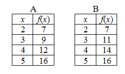
The two remaining tables were

Table MVT

Notice that in table A the values are increasing at an increasing rate, and in table B the values are increasing at a decreasing rate. Thus, table B is the correct choice. By the end of the year that kind of reasoning is enough for students to determine the correct answer.

Students could also draw a quick graph and see that table A was concave up and B was concave down. This will give them the correct answer, but technically it is a wrong approach since, once again, there is no way to know what happens between the values; we should not just connect the points and draw a conclusion.

The correct reasoning is based on the Mean Value Theorem (MVT).

In table A, by the MVT there must be a number c1 between 2 and 3 where {f}'\left( {{c}_{1}} \right)=2 the slope between the points (2,7) and (3, 9). Also, there must be a number c2 between 3 and 4 where {f}'\left( {{c}_{2}} \right)=3 the slope between (3, 9) and (4, 12), and likewise a number c3 between 4 and 5 where {f}'\left( {{c}_{3}} \right)=4.

Then applying the MVT to these values of {f}'\left( x \right), there must be a number, say d1 between c1 and c2 where {{f}'}'\left( {{d}_{1}} \right)=\frac{3-2}{{{c}_{2}}-{{c}_{1}}}>0. Since the second derivative should be negative everywhere, table A is eliminated making the remaining table B the correct choice.

If we do a similar analysis of Table B, we find that the MVT values for the second derivative are all negative. However, we cannot be sure this is true for all values of f in table B, since we can never be sure what happens between the values in a table. But table B is the only one that could be the one described since the others clearly are not.

In this post we saw how the MVT can be used in a numerical setting. I discussed the MVT in an analytic setting on September 28, 2012 and graphically on October 1, 2012.

The Mean Value Theorem II

The Rule of Four suggests that mathematics be studied from the analytical, graphical, numerical, and verbal points of view. Proof can only be done analytically – using symbols and equations. Graphs, numbers, and words aid in that, but do not by themselves prove anything.

On the other hand, numbers and especially graphs can make many of the theorems much more understandable and often can convince one of the truth of a theorem far better than the actual proof.

The Mean Value Theorem, MVT, is a good example; it can be demonstrated with a lot less trouble. See the figure above. Picture the blue line connecting the endpoints of the interval (the secant line) moving up, parallel to its original position. See the figure above. As this line moves up it intersects the graph twice, until eventually, just before it does not intersect at all, it comes to a place where it intersects exactly one. At this point it is tangent to the original graph. Since it is tangent, the slope of the line is the same as the derivative, {f}'\left( c \right), at that point.

So, the derivative is equal to the slope of the line between the endpoints. The MVT says that if its hypotheses are true, then there must be a place where the slope of the tangent line is parallel to the slope of the secant line.
But wait, there is more: at that point the instantaneous rate of change of the function is equal to the average rate of change over the interval.

This shows a real strength of looking at the graph.

But it is only one of many possible graphs. The graph could look like this figure:

Here there are several places (5 to be exact) where the tangent line is parallel to the secant line; there could be several on one side, or several on both sides. But this is not a problem; this does not contradict the MVT, which says there is at least one.

Yet another way to show the MVT is this. Near the left end of the first graph above the slope of the tangent to the graph (the derivative) is larger than the slope of the secant line; near the right end the slope of the tangent is less than the slope of the secant. So somewhere in between, by the Intermediate Value Theorem, the slope of the tangent must equal the slope of the secant. (For the purists out there, this is from Darboux’s theorem, and requires a slightly stronger hypothesis, namely that the one-sided derivatives at a and b exist.)

Rolle’s theorem can be demonstrated with either of these approaches as well. Rolle’s Theorem is really a special case of the MVT where the slope of the secant line is zero.

In conclusion, I think that this sequence of theorems is a good place to do a little proving of theorems. On the other hand you can easily show the results other ways. In fact, the method at the beginning of this post should be shown anyway in order to give students a good picture (no pun intended) of the MVT. It will help them remember what it is all about.

The Mean Value Theorem I

The Mean Value Theorem says that if a function, f , is continuous on a closed interval [a, b] and differentiable on the open interval (a, b) then there is a number c in the open interval (a, b) such that

\displaystyle {f}'\left( c \right)=\frac{f\left( b \right)-f\left( a \right)}{b-a}.

It says a lot more than that which we will consider in the next post.

The proof, which once you know where to start, is straight forward and rests on Rolle’s theorem.

In the figure above we see the graph of f and the graph of the (secant) line, y (x), between the endpoints of f. we define a new function h(x) = f (x) – y (x), this is the vertical distance from f to y. The equation of the line is in the figure and so

\displaystyle f\left( x \right)-f\left( a \right)-\frac{f\left( b \right)-f\left( a \right)}{b-a}\left( x-a \right)=h\left( x \right)

The function h meets all the conditions of Rolle’s theorem. In particular, h (a) = h (b) = 0 since at the endpoint the two graphs intersect and the distance between them is zero. You can also verify this by substituting first x = a and then x = b into h. Therefore, by Rolle’s theorem there is a number x = c between a and b such that {h}'\left( c \right)=0. So we’ll find the derivative and substitute in x = c.

\displaystyle {f}'\left( x \right)-0-\frac{f\left( b \right)-f\left( a \right)}{b-a}={h}'\left( x \right)

\displaystyle {f}'\left( c \right)-\frac{f\left( b \right)-f\left( a \right)}{b-a}=0

\displaystyle {f}'\left( c \right)=\frac{f\left( b \right)-f\left( a \right)}{b-a}

This last equation is very important and will come back in the second act and elsewhere.

So again, we see how one theorem, Rolle’s, leads to another, the MVT.

The arc from the definition of derivative, through Fermat’s theorem and Rolle’s theorem to the MVT is, I think, a good way to demonstrate how theorems and their proofs work together. Since I would not like my students not to have any familiarity with proof and definition, I think this is a good place to show them just a little of what it’s all about.

On the other hand, we have ended up with a strange equation, which apparently has something to do with mean value, whatever that is. In the final post in this series we will discuss what this all means and how to convince your students of the truth of the MVT without all the symbol pushing that’s required in a proof.

I don’t like this proof because you must know to set up the function h at the beginning. It is “legal” to do that, but how do you know to do it? On the other hand, doing things like that is something that has to be done sometimes and students need to know this too. But we’ll see an easier way in the next post.