The Mean Value Theorem says that if a function, f , is continuous on a closed interval [a, b] and differentiable on the open interval (a, b) then there is a number c in the open interval (a, b) such that

.

It says a lot more than that which we will consider in the next post.

The proof, which once you know where to start, is straight forward and rests on Rolle’s theorem.

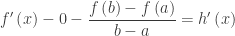
In the figure above we see the graph of f and the graph of the (secant) line, y (x), between the endpoints of f. we define a new function h(x) = f (x) – y (x), this is the vertical distance from f to y. The equation of the line is in the figure and so

The function h meets all the conditions of Rolle’s theorem. In particular, h (a) = h (b) = 0 since at the endpoint the two graphs intersect and the distance between them is zero. You can also verify this by substituting first x = a and then x = b into h. Therefore, by Rolle’s theorem there is a number x = c between a and b such that . So we’ll find the derivative and substitute in x = c.

This last equation is very important and will come back in the second act and elsewhere.

So again, we see how one theorem, Rolle’s, leads to another, the MVT.

The arc from the definition of derivative, through Fermat’s theorem and Rolle’s theorem to the MVT is, I think, a good way to demonstrate how theorems and their proofs work together. Since I would not like my students not to have any familiarity with proof and definition, I think this is a good place to show them just a little of what it’s all about.

On the other hand, we have ended up with a strange equation, which apparently has something to do with mean value, whatever that is. In the final post in this series we will discuss what this all means and how to convince your students of the truth of the MVT without all the symbol pushing that’s required in a proof.

I don’t like this proof because you must know to set up the function h at the beginning. It is “legal” to do that, but how do you know to do it? On the other hand, doing things like that is something that has to be done sometimes and students need to know this too. But we’ll see an easier way in the next post.