Open or Closed?

About this time of year, you find someone, hopefully one of your students, asking, “If I’m finding where a function is increasing, is the interval open or closed?”

Do you have an answer?

This is a good time to teach some things about definitions and theorems.

The place to start is to ask what it means for a function to be increasing. Here is the definition:

A function is increasing on an interval if, and only if, for all (any, every) pairs of numbers x1 < x2 in the interval, f(x1) < f(x2).”

(For decreasing on an interval, the second inequality changes to f(x1) > f(x2). All of what follows applies to decreasing with obvious changes in the wording.)

  1. Notice that functions increase or decrease on intervals, not at individual points. We will come back to this in a minute.
  2. Numerically, this means that for every possible pair of points, the one with the larger x-value always produces a larger function value.
  3. Graphically, this means that as you move to the right along the graph, the graph is going up.
  4. Analytically, this means that we can prove the inequality in the definition.

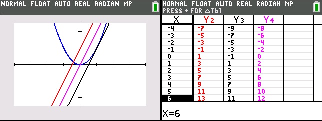
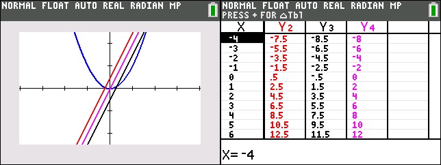
For an example of this last point consider the function f(x) = x2. Let x2 = x1 + h where h > 0. Then in order for f(x1) < f(x2) it must be true that

\displaystyle {{x}_{1}}^{2}<{{\left( {{{x}_{1}}+h} \right)}^{2}}

\displaystyle 0<{{\left( {{{x}_{1}}+h} \right)}^{2}}-{{x}_{1}}^{2}

\displaystyle 0<{{x}_{1}}^{2}+2{{x}_{1}}h+{{h}^{2}}-{{x}_{1}}^{2}

\displaystyle 0<2{{x}_{1}}h+{{h}^{2}}

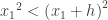
This can only be true if \displaystyle {{x}_{1}}\ge 0 Thus, x2 is increasing only if\displaystyle {{x}_{1}}\ge 0

Now, of course, we rarely, if ever, go to all that trouble. And it is even more trouble for a function that increases on several intervals.  The usual way of finding where a function is increasing is to look at its derivative.

Notice that the expression \displaystyle 0<{{x}_{1}}^{2}+2{{x}_{1}}h+{{h}^{2}}-{{x}_{1}}^{2} looks a lot like the numerator of the original limit definition of the derivative of x2 at x = x1, namely \displaystyle 0<{{\left( {{{x}_{1}}+h} \right)}^{2}}-{{x}_{1}}^{2}. If h > 0, where the function is increasing the numerator is positive and the derivative is positive also. Turning this around we have a theorem that says, If \displaystyle {f}'\left( {{{x}_{1}}} \right)>0 for all x in an interval, then the function is increasing on the interval. That makes it much easier to find where a function is increasing, we simplify find where its derivative is positive.

There is only a slight problem in that the theorem does not say what happens if the derivative is zero somewhere on the interval. If that is the case, we must go back to the definition of increasing on an interval or use a different method. For example, the function x3 is increasing everywhere, even though its derivative at the origin is zero.

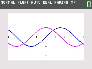
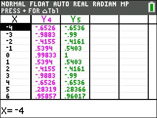
Let’s consider another example. The function sin(x) is increasing on the interval \displaystyle [-\tfrac{\pi }{2},\tfrac{\pi }{2}] (among others) and decreasing on \displaystyle [\tfrac{\pi }{2},\tfrac{3\pi }{2}]. It bothers some that \displaystyle \tfrac{\pi }{2} is in both intervals and that the derivative of the function is zero at x = \displaystyle \tfrac{\pi }{2}. This is not a problem. Sin(\displaystyle \tfrac{\pi }{2}) is larger than all the other values is both intervals, so by the definition, and not the theorem, the intervals are correct.

It is generally true that if a function is continuous on the closed interval [a,b] and increasing on the open interval (a,b) then it must be increasing on the closed interval [a,b] as well.

Returning to the first point above: functions increase or decrease on intervals not at points. You do find questions in books and on tests that ask, “Is the function increasing at x = a.” The best answer is to humor them and answer depending on the value of the derivative at that point. Since the derivative is a limit as h approaches zero, the function must be defined on some interval around x = a in which h is approaching zero. So, answer according to the value of the derivative on that interval.

You can find more on this here.

Case Closed.

Slightly revised from a posted published on November 2, 2012.

Advertisement

Unit 2 – Definition of the Derivative

This is a re-post and update of the second in a series of posts from last year. It contains links to posts on this blog about the definition of the derivative for your reference in planning. Other updated post on the 2019 CED will come throughout the year, hopefully, a few weeks before you get to the topic. 

Unit 2 contains topics rates of change, difference quotients, and the definition of the derivative (CED – 2019 p. 51 – 66). These topics account for about 10 – 12% of questions on the AB exam and 4 – 7% of the BC questions.

Topics 2.1 – 2.4: Introducing and Defining the Derivative 

Topic 2.1: Average and Instantaneous Rate of Change. The forward difference quotient is used to introduce the idea of rate of change over an interval and its limit as the length of the interval approaches zero is the instantaneous rate of change.

Topic 2.2: Defining the derivative and using derivative notation. The derivative is defined as the limit of the difference quotient from topic 1 and several new notations are introduced. The derivative is the slope of the tangent line at a point on the graph. Explain graphically, numerically, and analytically how the three representations relate to each other and the slope.

Topic 2.3 Estimating the derivative at a point.  Using tables and technology to approximate derivatives is used in this topic. The two resources in the sidebar will be helpful here.

Topic 2.4: Differentiability and Continuity. An important theorem is that differentiability implies continuity – everywhere a function is differentiable it is continuous.  Its converse is false – a function may be continuous at a point, but not differentiable there. A counterexample is the absolute value function, |x|, at x = 0.

One way that the definition of derivative is tested on recent exams which bothers some students is to ask a limit like

displaystyle underset{{xto 0}}{mathop{{lim }}},frac{{tan left( {tfrac{pi }{4}+x} right)-tan left( {tfrac{pi }{4}} right)}}{x}.

From the form of the limit students should realize this as the limit definition of the derivative. The h in the definition has been replaced by x. The function is tan(x) at the point where displaystyle a=tfrac{pi }{4}. The limit is displaystyle {{sec }^{2}}left( {tfrac{pi }{4}} right)=2.

Topics 2.5 – 2.10: Differentiation Rules

The remaining topics in this chapter are the rules for calculating derivatives without using the definition. These rules should be memorized as students will be using them constantly. There will be additional rules in Unit 3 (Chain Rule, Implicit differentiation, higher order derivative) and for BC, Unit 9 (parametric and vector equations).

Topic 2.5: The Power Rule

Topic 2.6: Constant, sum, difference, and constant multiple rules

Topic 2.7: Derivatives of the cos(x), sin(x), ex, and ln(x). This is where you use the squeeze theorem.

Topic 2.8. The Product Rule

Topic 2.9: The Quotient Rule

Topic 2.10: Derivative of the other trigonometric functions

The rules can be tested directly by just asking for the derivative or its value at a point for a given function. Or they can be tested by requiring the students to use the rule of an general expression and then find the values from a table, or a graph. See 2019 AB 6(b)


The suggested number of 40 – 50 minute class periods is 13 – 14 for AB and 9 – 10  for BC. This includes time for testing etc. Topics 2.1, 2,2, and 2.3 kind of flow together, but are important enough that you should spend time on them so that students develop a good understanding of what a derivative is. Topics 2.5 thru 2.10 can be developed in 2 -3 days, but then time needs to be spent deciding which rule(s) to use and in practice using them. The sidebar resource in the CED on “Selecting Procedures for Derivative” may be helpful here.


Other post on these topics

DEFINITION OF THE DERIVATIVE

Local Linearity 1  The graphical manifestation of differentiability with pathological examples.

Local Linearity 2   Using local linearity to approximate the tangent line. A calculator exploration.

Discovering the Derivative   A graphing calculator exploration

The Derivative 1  Definition of the derivative

The Derivative 2   Calculators and difference quotients

Difference Quotients 1

Difference Quotients II

Tangents and Slopes

       Differentiability Implies Continuity

Adapting 2021 AB 4 / BC 4

FINDING DERIVATIVES 

Why Radians?  Don’t do calculus without them

The Derivative Rules 1  Constants, sums and differences, powers.

The Derivative Rules 2  The Product rule

The Derivative Rules 3  The Quotient rule


Here are links to the full list of posts discussing the ten units in the 2019 Course and Exam Description.the 2019 versions.

2019 CED – Unit 1: Limits and Continuity

2019 CED – Unit 2: Differentiation: Definition and Fundamental Properties.

2019 CED – Unit 3: Differentiation: Composite , Implicit, and Inverse Functions

2019 CED – Unit 4 Contextual Applications of the Derivative  Consider teaching Unit 5 before Unit 4

2019 – CED Unit 5 Analytical Applications of Differentiation  Consider teaching Unit 5 before Unit 4

2019 – CED Unit 6 Integration and Accumulation of Change

2019 – CED Unit 7 Differential Equations  Consider teaching after Unit 8

2019 – CED Unit 8 Applications of Integration   Consider teaching after Unit 6, before Unit 7

2019 – CED Unit 9 Parametric Equations, Polar Coordinates, and Vector-Values Functions 

2019 CED Unit 10 Infinite Sequences and Series


Definition of the Derivative – Unit 2

This is a re-post and update of the second in a series of posts from last year. It contains links to posts on this blog about the definition of the derivative for your reference in planning. Other updated post on the 2019 CED will come throughout the year, hopefully, a few weeks before you get to the topic. 

Unit 2 contains topics rates of change, difference quotients, and the definition of the derivative (CED – 2019 p. 51 – 66). These topics account for about 10 – 12% of questions on the AB exam and 4 – 7% of the BC questions.

Topics 2.1 – 2.4: Introducing and Defining the Derivative 

Topic 2.1: Average and Instantaneous Rate of Change. The forward difference quotient is used to introduce the idea of rate of change over an interval and its limit as the length of the interval approaches zero is the instantaneous rate of change.

Topic 2.2: Defining the derivative and using derivative notation. The derivative is defined as the limit of the difference quotient from topic 1 and several new notations are introduced. The derivative is the slope of the tangent line at a point on the graph. Explain graphically, numerically, and analytically how the three representations relate to each other and the slope.

Topic 2.3 Estimating the derivative at a point.  Using tables and technology to approximate derivatives is used in this topic. The two resources in the sidebar will be helpful here.

Topic 2.4: Differentiability and Continuity. An important theorem is that differentiability implies continuity – everywhere a function is differentiable it is continuous.  Its converse is false – a function may be continuous at a point, but not differentiable there. A counterexample is the absolute value function, |x|, at x = 0.

One way that the definition of derivative is tested on recent exams which bothers some students is to ask a limit like

\displaystyle \underset{{x\to 0}}{\mathop{{\lim }}}\,\frac{{\tan \left( {\tfrac{\pi }{4}+x} \right)-\tan \left( {\tfrac{\pi }{4}} \right)}}{x}.

From the form of the limit students should realize this as the limit definition of the derivative. The h in the definition has been replaced by x. The function is tan(x) at the point where \displaystyle a=\tfrac{\pi }{4}. The limit is \displaystyle {{\sec }^{2}}\left( {\tfrac{\pi }{4}} \right)=2.

Topics 2.5 – 2.10: Differentiation Rules

The remaining topics in this chapter are the rules for calculating derivatives without using the definition. These rules should be memorized as students will be using them constantly. There will be additional rules in Unit 3 (Chain Rule, Implicit differentiation, higher order derivative) and for BC, Unit 9 (parametric and vector equations).

Topic 2.5: The Power Rule

Topic 2.6: Constant, sum, difference, and constant multiple rules

Topic 2.7: Derivatives of the cos(x), sin(x), ex, and ln(x). This is where you use the squeeze theorem.

Topic 2.8. The Product Rule

Topic 2.9: The Quotient Rule

Topic 2.10: Derivative of the other trigonometric functions

The rules can be tested directly by just asking for the derivative or its value at a point for a given function. Or they can be tested by requiring the students to use the rule of an general expression and then find the values from a table, or a graph. See 2019 AB 6(b)


The suggested number of 40 – 50 minute class periods is 13 – 14 for AB and 9 – 10  for BC. This includes time for testing etc. Topics 2.1, 2,2, and 2.3 kind of flow together, but are important enough that you should spend time on them so that students develop a good understanding of what a derivative is. Topics 2.5 thru 2.10 can be developed in 2 -3 days, but then time needs to be spent deciding which rule(s) to use and in practice using them. The sidebar resource in the CED on “Selecting Procedures for Derivative” may be helpful here.


Other post on these topics

DEFINITION OF THE DERIVATIVE

Local Linearity 1  The graphical manifestation of differentiability with pathological examples.

Local Linearity 2   Using local linearity to approximate the tangent line. A calculator exploration.

Discovering the Derivative   A graphing calculator exploration

The Derivative 1  Definition of the derivative

The Derivative 2   Calculators and difference quotients

Difference Quotients 1

Difference Quotients II

Tangents and Slopes

         Differentiability Implies Continuity

FINDING DERIVATIVES 

Why Radians?  Don’t do calculus without them

The Derivative Rules 1  Constants, sums and differences, powers.

The Derivative Rules 2  The Product rule

The Derivative Rules 3  The Quotient rule


Here are links to the full list of posts discussing the ten units in the 2019 Course and Exam Description.the 2019 versions.

2019 CED – Unit 1: Limits and Continuity

2019 CED – Unit 2: Differentiation: Definition and Fundamental Properties.

2019 CED – Unit 3: Differentiation: Composite , Implicit, and Inverse Functions

2019 CED – Unit 4 Contextual Applications of the Derivative  Consider teaching Unit 5 before Unit 4

2019 – CED Unit 5 Analytical Applications of Differentiation  Consider teaching Unit 5 before Unit 4

2019 – CED Unit 6 Integration and Accumulation of Change

2019 – CED Unit 7 Differential Equations  Consider teaching after Unit 8

2019 – CED Unit 8 Applications of Integration   Consider teaching after Unit 6, before Unit 7

2019 – CED Unit 9 Parametric Equations, Polar Coordinates, and Vector-Values Functions 

2019 CED Unit 10 Infinite Sequences and Series


Differentiability Implies Continuity

An important theorem concerning derivatives is this:

If a function f is differentiable at x = a, then f is continuous at x = a.

The proof begins with the identity that for all x\ne a

\displaystyle f\left( x \right)-f\left( a \right)=\left( {x-a} \right)\frac{{f\left( x \right)-f\left( a \right)}}{{x-a}}

\displaystyle \underset{{x\to a}}{\mathop{{\lim }}}\,\left( {f\left( x \right)-f\left( a \right)} \right)=\underset{{x\to a}}{\mathop{{\lim }}}\,\left( {\left( {x-a} \right)\frac{{f\left( x \right)-f\left( a \right)}}{{x-a}}} \right)=\underset{{x\to a}}{\mathop{{\lim }}}\,\left( {x-a} \right)\cdot \underset{{x\to a}}{\mathop{{\lim }}}\,\frac{{f\left( x \right)-f\left( a \right)}}{{x-a}}

\displaystyle \underset{{x\to a}}{\mathop{{\lim }}}\,\left( {f\left( x \right)-f\left( a \right)} \right)=0\cdot {f}'\left( a \right)=0

And therefore, \underset{{x\to a}}{\mathop{{\lim }}}\,f\left( x \right)=f\left( a \right)

Since both sides are finite, the function is continuous at x = a.


The converse of this theorem is false: A continuous function is not necessarily differentiable. A counterexample is the absolute value function which is continuous at the origin but not differentiable there. (The slope approaching from the left is not equal to the slope from the right.)

This is a theorem whose contrapositive is used as much as the theorem itself. The contrapositive is,

If a function is not continuous at a point, then it is not differentiable there.

Example 1: A function such as  \displaystyle g\left( x \right)=\frac{{{{x}^{2}}-9}}{{x-3}} has a (removable) discontinuity at x = 3, but no value there.

So, in the limit definition of the derivative, \displaystyle \text{ }\!\!~\!\!\text{ }\underset{{h\to 0}}{\mathop{{\lim }}}\,\frac{{g\left( {3+h} \right)-g\left( 3 \right)}}{h} there is no value of g(3) to use, and the derivative does not exist.

Example 2:  \displaystyle f\left( x \right)=\left\{ {\begin{array}{*{20}{c}} {{{x}^{2}}} & {x\le 1} \\ {{{x}^{2}}+3} & {x>1} \end{array}} \right.
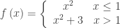
. This function has a jump discontinuity at x = 1.

Since the point (1, 1) is on the left part of the graph, if h > 0, f\left( {1+h} \right)-f\left( 1 \right)>3 and the limit  will always be a number greater than 3 divided by zero and will not exist. Therefore, even though the slopes from both side of x =1 approach the same value, namely 2, the derivative does not exist at x = 1.

This also applies to a situation like example 1 if f(3) were some value that did not fill in the hole in the graph.


On the AP Calculus exams students are often asked about the derivative of a function like those in the examples, and the lack of continuity should be an immediate clue that the derivative does not exist. See 2008 AB 6 (multiple-choice).

Just as important are questions in which the function is given as differentiable, but the student needs to know about continuity. Just remember: differentiability implies continuity. See 2013 AB 14 in which you must realize the since the function is given as differentiable at x = 1, it must be continuous there to solve the problem.


Continuity of the Derivative

A question that comes up is, if a function is differentiable is its derivative differentiable? The answer is no. While almost always the derivative is also differentiable, there is this counterexample:

\displaystyle f\left( x \right)=\left\{ {\begin{array}{*{20}{c}} {{{x}^{2}}\sin \left( {\frac{1}{x}} \right)} & {x\ne 0} \\ 0 & {x=0} \end{array}} \right.

The first line of the function has a removable oscillating discontinuity at x = 0, but since the \displaystyle {{x}^{2}} factor squeezes the function to the origin; the added condition that \displaystyle f\left( 0 \right)=0 makes the function continuous. Differentiating gives

\displaystyle {{f}^{'}}\left( x \right)={{x}^{2}}\cos \left( {\frac{1}{x}} \right)\left( {\frac{{-1}}{{{{x}^{2}}}}} \right)+2x\sin \left( {\frac{1}{x}} \right)=-\cos \left( {\frac{1}{x}} \right)+2x\sin \left( {\frac{1}{x}} \right)

And now there is no way to get around the oscillating discontinuity at x = 0.


2019 CED – Unit 2: Differentiation: Definition and Fundamental Properties.

Unit 2 contains topics rates of change, difference quotients, and the definition of the derivative (CED – 2019 p. 51 – 66). These topics account for about 10 – 12% of questions on the AB exam and 4 – 7% of the BC questions.

Topics 2.1 – 2.4: Introducing and Defining the Derivative 

Topic 2.1: Average and Instantaneous Rate of Change. The forward difference quotient is used to introduce the idea of rate of change over an interval and its limit as the length of the interval approaches zero is the instantaneous rate of change.

Topic 2.2: Defining the derivative and using derivative notation. The derivative is defined as the limit of the difference quotient from topic 1 and several new notations are introduced. The derivative is the slope of the tangent line at a point on the graph. Explain graphically, numerically, and analytically how the three representations relate to each other and the slope.

Topic 2.3 Estimating the derivative at a point.  Using tables and technology to approximate derivatives is used in this topic. The two resources in the sidebar will be helpful here.

Topic 2.4: Differentiability and Continuity. An important theorem is that differentiability implies continuity – everywhere a function is differentiable it is continuous.  Its converse is false – a function may be continuous at a point, but not differentiable there. A counterexample is the absolute value function, |x|, at x = 0.

One way that the definition of derivative is tested on recent exams which bothers some students is to ask a limit like

\displaystyle \underset{{x\to 0}}{\mathop{{\lim }}}\,\frac{{\tan \left( {\tfrac{\pi }{4}+x} \right)-\tan \left( {\tfrac{\pi }{4}} \right)}}{x}.

From the form of the limit students should realize this as the limit definition of the derivative. The h in the definition has been replaced by x. The function is tan(x) at the point where \displaystyle a=\tfrac{\pi }{4}. The limit is \displaystyle {{\sec }^{2}}\left( {\tfrac{\pi }{4}} \right)=2.

Topics 2.5 – 2.10: Differentiation Rules

The remaining topics in this chapter are the rules for calculating derivatives without using the definition. These rules should be memorized as students will be using them constantly. There will be additional rules in Unit 3 (Chain Rule, Implicit differentiation, higher order derivative) and for BC, Unit 9 (parametric and vector equations).

Topic 2.5: The Power Rule

Topic 2.6: Constant, sum, difference, and constant multiple rules

Topic 2.7: Derivatives of the cos(x), sin(x), ex, and ln(x). This is where you use the squeeze theorem.

Topic 2.8. The Product Rule

Topic 2.9: The Quotient Rule

Topic 2.10: Derivative of the other trigonometric functions

The rules can be tested directly by just asking for the derivative or its value at a point for a given function. Or they can be tested by requiring the students to use the rule of an general expression and then find the values from a table, or a graph. See 2019 AB 6(b)


The suggested number of 40 – 50 minute class periods is 13 – 14 for AB and 9 – 10  for BC. This includes time for testing etc. Topics 2.1, 2,2, and 2.3 kind of flow together, but are important enough that you should spend time on them so that students develop a good understanding of what a derivative is. Topics 2.5 thru 2.10 can be developed in 2 -3 days, but then time needs to be spent deciding which rule(s) to use and in practice using them. The sidebar resource in the CED on “Selecting Procedures for Derivative” may be helpful here.


Other post on these topics

DEFINITION OF THE DERIVATIVE

Local Linearity 1  The graphical manifestation of differentiability with pathological examples.

Local Linearity 2   Using local linearity to approximate the tangent line. A calculator exploration.

Discovering the Derivative   A graphing calculator exploration

The Derivative 1  Definition of the derivative

The Derivative 2   Calculators and difference quotients

Difference Quotients 1

Difference Quotients II

Tangents and Slopes

         Differentiability Implies Continuity

FINDING DERIVATIVES 

Why Radians?  Don’t do calculus without them

The Derivative Rules 1  Constants, sums and differences, powers.

The Derivative Rules 2  The Product rule

The Derivative Rules 3  The Quotient rule


Here are links to the full list of posts discussing the ten units in the 2019 Course and Exam Description.

2019 CED – Unit 1: Limits and Continuity

2019 CED – Unit 2: Differentiation: Definition and Fundamental Properties.

2019 CED – Unit 3: Differentiation: Composite , Implicit, and Inverse Functions

2019 CED – Unit 4 Contextual Applications of the Derivative  Consider teaching Unit 5 before Unit 4

2019 – CED Unit 5 Analytical Applications of Differentiation  Consider teaching Unit 5 before Unit 4

2019 – CED Unit 6 Integration and Accumulation of Change

2019 – CED Unit 7 Differential Equations  Consider teaching after Unit 8

2019 – CED Unit 8 Applications of Integration   Consider teaching after Unit 6, before Unit 7

2019 – CED Unit 9 Parametric Equations, Polar Coordinates, and Vector-Values Functions 

2019 CED Unit 10 Infinite Sequences and Series


Local Linearity

If you use your calculator or graphing program and zoom-in of the graph of a function (with equal zoom factors in both directions), the graph eventually looks like a line: the graph appears to be straight. This property is called Local Linearity. The slope of this line is the number called the derivative. (There are exceptions: if the graph never appears linear, then no derivative exists at that point.) Local Linearity is the graphical manifestation of differentiability. 

To find this slope, we need to zoom-in numerically. Zooming-in numerically is accomplished by finding the slope of a secant line, a line that intersects the graph twice near the point we are interested in. Then finding the limit of that slope as the two points come closer to our point. This limit is the derivative. It is also the slope of the line tangent to the function at the point. 

While limit is what makes all of the calculus work, people usually think of calculus as starting with the derivative. The first problem in calculus is finding the slope of a line tangent to a graph at a point and then writing the equation of that tangent line. The slope is called the derivative and a function whose derivative exists is said to be differentiable. 

This week’s posts start with local linearity and tangent lines. They lead to the difference quotient and the equation of the tangent line.

Local Linearity I

Local Linearity II      Working up to difference quotient. The next post explains this in more detail.

Tangent Lines approaching difference quotients on calculator by graphing tan line.

Next week: Difference Quotients.


Revised from a post of August 29, 2017


Seeing Difference Quotients

Third in the graphing calculator series. 

In working up to the definition of the derivative you probably mention difference quotients. They are

The forward difference quotient (FDQ): \displaystyle \frac{f\left( x+h \right)-f\left( x \right)}{h}

The backwards difference quotient (BDQ): \displaystyle \frac{f\left( x \right)-f\left( x-h \right)}{h}, and

The symmetric difference quotient (SDQ): \displaystyle \frac{f\left( x+h \right)-f\left( x-h \right)}{2h}

Each of these is the slope of a (different) secant line and the limit of each as, if it exists, is the same and is the derivative of the function f at the point (x, f(x)). (We will assume h > 0 although this is not really necessary; if h < 0 the FDQ becomes the BDQ and vice versa.)

To see how this works you can graph a function and the three difference quotients on a graphing calculator. Here is how. Enter the function as the first function on your calculator and the difference quotients with it. Each of the difference quotients is defined in terms of Y1; this allows us to investigate the difference quotients of different functions by changing only Y1.

DQ 1

Now, on the home screen assign a value to h by typing [1] [STO] [alpha] [h]

Graph the result in a square window.

The look at the table screen. (Y1 has been turned off). Can you express Y2, Y3, and Y4 in term of x?

DQ 2

Then change h by storing a different value, say ½, to h and graph again. Then look at the table screen again. Can you express Y2, Y3, and Y4 in term of x?

DQ 3

Then graph again with h = -0.1

DQ 4

As you can see as h gets smaller (h 0), the three difference quotients are FDQ: 2x + h, the BDQ is 2x – h, and the SDQ is 2x. They converge to the same thing. The limit of each difference quotient as h approaches zero is twice the x coordinate of the point. If you’re not sure try a smaller value of h.

The function to which each of these converge is called the derivative of the original function (Y1). In the example the derivative of x2 is 2x.

Now try another function say, Y1 = sin(x) and repeat the graphs and tables above. The tables will probably not be of much help, since the pattern is not familiar. The graph shows the function (dark blue) and only the SDQ (light blue), h = 0.1 Can you guess what the derivative might be?

DQ 5

I f you guessed cos(x) you are correct. The table shows the SDQ values as Y4, and the values of cos(x) as Y5. Pretty close! If you want to get closer try h = 0.001.

DQ 6

If you have a CAS calculators such as the TI-Nspire or the HP PRIME you can do this activity with sliders. Also you may try this with DESMOS. Click here or on the graph below. Some interesting functions to start with are cos(x) and | x |.

And by the way, the SDQ is what most graphing calculators use to calculate the derivative. It is called nDeriv on TI calculators.