AP Calculus Review 2023

For several years now, I’ve been posting a series of notes on reviewing for the AP Calculus Exams. The questions on the AP Calculus exams, both multiple-choice and free response, fall into ten types. I’ve published posts on each. The ten types have not changed over the years, so there is not much to add. They are updated from time to time. The posts may be found under the “Blog Guide” tab above: click on AP Exam Review. The same links are below with a brief explanation of each.

I hope these will help as you review for this year’s exam.

General information and suggestions

  • AP Exam Review – Suggestions, hints, information, and other resources for reviewing. How to get started. What to tell your students. Simulated (mock) exams.
  • To dx or not dx – Yes, use past exams and the scoring guideline to review, but don’t worry about the fine points of scoring; be more stringent than the readers.
  • Practice Exams – A Modest Proposal Like it or not (and the AP folks certainly do not) the answers are all online. What to do about that. Don’t overlook the replies at the end of this post.

The Ten Type Questions.

Other than simply finding a limit, a derivative, an antiderivative, or evaluating a definite integral, the AP Calculus exam questions fall into these ten types. These are different from the ten units in the CED. Students are often expected to use knowledge from more than one unit in a single question.

These posts outline what each type of question covers and what students should be able to do. They include references to good questions, free-response and multiple-choice, and links to other posts on the topic.

  • Type 3 questions – Graph analysis. Given the derivative often as a graph, students must answer questions about the function – extreme values, increasing, decreasing, concavity, etc.
  • Type 6 questions – Differential equations. Students are asked to solve a first-order separable differential equation, work with a slope field, or other related ideas. BC students may be asked to use Euler’s Method to approximate a value and discuss the logistic equation.
  • Type 7 questions – Miscellaneous. These include finding the first and second derivative of implicitly defined relation, solving a related rate problem or other topics not included in the other types.
  • Type 10 questions – Sequences and Series (BC topic) Questions ask student to determine the convergence of series using various convergence tests and to write and work with a Taylor and Maclaurin series, find its radius and interval of convergence.

Also, Calc-Medic has posted a searchable database of all the AP Calculus Free-response questions from 1998 on. The link is here. While you’re there take a look at their website which has lots of resources and free lesson plans. For mor on Calc-medic see this post.

This year’s exam will be given on Monday May 8, 2023, at 8:00 am local time.


Update March 9, 2023 – Calc-medic

Advertisement

Visualizing Unit 9

As you probably realize by now, I think graphs, drawing and other visuals are a great aid in teaching and learning mathematics. Desmos is a free graphing app that many teachers and students use to graph and make other illustrations. Demonstrations can be made in advance and shared with students and other teachers.

Recently, I was looking a some material from Unit 9 Parametric Equation, Polar Coordinates, and Vector-Valued Functions, BC topics, from the current AP Calculus CED. I ended up making three new Desmos illustrations for use in this unit. They will also be useful in a precalculus course introducing these topics. Hope you find them helpful.

Polar Graph Demo

Link

You may replace the polar equation with any polar equation you are interested in. There are directions in the demo. Moving the “a” slider will show a ray rotating around the pole. The “a” value is the angle, \displaystyle \theta 
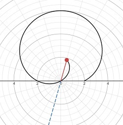
, in radians between the ray and the polar axis. On the ray is a segment with a point at its end. This segment’s length is \displaystyle \left| {r\left( \theta \right)} \right|. As you rotate the ray you can see the polar graph drawn. When \displaystyle r(\theta )<0 the segment extend in the opposite direction from the ray.

This demo may be used to introduce or review how polar equation work. An interesting extension is to enter something for the argument of the function that is not an integer muntiple of \displaystyle \theta and extend the domain past \displaystyle 2\pi , for example \displaystyle r=2+4\sin (1.2\theta )

Basic Parametric and Vector Demo

LInk

A parametric equation and the vector equation of the same curve differ only in notation. So, this demo works for both. Following the directions in the demo, you may see the graph being drawn using the “a” slider. You may turn on (1) the position vector and its components, (2) add the velocity vector attached to the moving point and “pulling” it to its new position, and (3) the acceleration vector “pulling” the velocity vector.

You may enter any parametric/vector equation. When you do, you will also have to enter its first and second derivative. Follow the directions in the demonstration.

Cycloids and their vectors

Link

This demo shows the path on a rolling wheel called a cycloid. The “a” slider moves the position of the point on the wheel. The point may be on the rim of the wheel (\displaystyle a=r
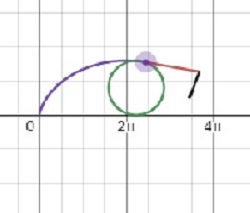
, on the interior of the wheel (\displaystyle a<r), or outside the wheel (\displaystyle a>r  – think the flange on a train wheel). Use the “u” slider to animate the drawing. The velocity and acceleration vectors are shown; they may be turned off. The velocity vector is tangent to the curve (not to the circle) and seems to “pull” the point along the curve. The acceleration vector “pulls” the velocity vector. The equation in this demo should not be changed.

The last two demonstrations give a good idea of how the velocity and acceleration vectors affect the movement of the point.

Hope you find these helpful.

.

Differential Equations (Type 6)

AP Questions Type 6: Differential Equations

Differential equations are tested in the free-response section of the AP exams almost every year. The actual solving of the differential equation is usually the main part of the problem accompanied by a related question such as a slope field or a tangent line approximation. BC students may also be asked to approximate using Euler’s Method. Several parts of the BC questions are often suitable for AB students and contribute to the AB sub-score of the BC exam. This topic may also appear in the multiple-choice sections of the exams. What students should be able to do
  • Find the general solution of a differential equation using the method of separation of variables (this is the only method tested).
  • Find a particular solution using the initial condition to evaluate the constant of integration – initial value problem (IVP).
  • Determine the domain restrictions on the solution of a differential equation. See this post for more on the domain of a differential equation.
  • Understand that proposed solution of a differential equation is a function (not a number) and if it and its derivative are substituted into the given differential equation the resulting equation is true. This may be part of doing the problem even if solving the differential equation is not required (see 2002 BC 5 – parts a, b and d are suitable for AB)
  • Growth-decay problems.
  • Draw a slope field by hand.
  • Sketch a particular solution on a given slope field.
  • Interpret a slope field.
  • Multiple-choice: Given a differential equation, identify is slope field.
  • Multiple-choice: Given a slope field identify its differential equation.
  • Use the given derivative to analyze a function such as finding extreme values
  • For BC only: Use Euler’s Method to approximate a solution.
  • For BC only: use the method of partial fractions to find the antiderivative after separating the variables.
  • For BC only: understand the logistic growth model, its asymptotes, meaning, etc. The exams so far, have never asked students to actually solve a logistic equation IVP
Look at the scoring standards to learn how the solution of the differential equation is scored, and therefore, how students should present their answer. This is usually the one free-response answer with the most points riding on it. Starting in 2016 the scoring has changed slightly. The five points are now distributed this way:
  • one point for separating the variables
  • one point each for finding the antiderivatives
  • one point for including the constant of integration and using the initial condition – that is, for writing “+ C” on the paper with one of the antiderivatives and substituting the initial condition; finding the value of C is included in the “answer point.” (In the older exams one point was earned for writing the +C and another point for using the initial condition.)
  • one point for solving for y: the “answer point”, for the correct answer. This point includes all the algebra and arithmetic in the problem including solving for C.
In the past, the domain of the solution was often included on the scoring standard, but unless it was specifically asked for in the question students did not need to include it. However, the CED. lists “EK 3.5A3 Solutions to differential equations may be subject to domain restrictions.” Perhaps this will be asked in the future. For more on domain restrictions with examples see this post. Shorter questions on this concept appear in the multiple-choice sections. As always, look over as many questions of this kind from past exams as you can find. For some previous posts on differential equations see January 5, 2015, and for post on related subjects see November 26, 2012, January 21, 2013, February 16, 2013 The Differential Equation question covers topics in Unit 7 of the CED.
Free-response examples:
  • 2019 There was no DE question in the free-response. You may assume the topic was tested in the multiple-choice sections.
  • 2017 AB4/BC4,
  • 2016 AB 4, BC 4, (different questions)
  • 2015 AB4/BC4,
  • 2013 BC 5
  • and a favorite Good Question 2 and Good Question 2 Continued
  • 2021 AB 6, BC 5 (b), (c)
  • 2022 AB5 – sketch solution on slope field, tangent line approximation, solve separable equation.
Multiple-choice examples from non-secure exams:
  • 2012 AB 23, 25
  • 2012 BC: 12, 14, 16, 23

Previous posts on these topics for both AB and BC include:

Differential Equations  A summary of the terms and techniques of differential equations and the method of separation of variables Domain of a Differential Equation – On domain restrictions. Accumulation and Differential Equations  Slope Fields An Exploration in Differential Equations An exploration illustrating many of the ideas of differential equations. The exploration is here in PDF form and the solution is here. The ideas include: finding the general solution of the differential equation by separating the variables, checking the solution by substitution, using a graphing utility to explore the solutions for all values of the constant of integration, finding the solutions’ horizontal and vertical asymptotes, finding several particular solutions, finding the domains of the particular solutions, finding the extreme value of all solutions in terms of C, finding the second derivative (implicit differentiation), considering concavity, and investigating a special case or two.

Previous Posts on BC Only Topics

Euler’s Method Euler’s Method for Making Money The Logistic Equation  Logistic Growth – Real and Simulated


Revised 2/20/2021, March 29, May 14, 2022

Riemann Sum & Table Problems (Type 5)

AP Questions Type 5: Riemann Sum & Table Problems

Information given in tables may be used to test a variety of ideas in calculus including analysis of functions, accumulation, theory and theorems, and position-velocity-acceleration, among others. Numbers and working with numbers are part of the Rule of Four and table problems are one way they are tested. This question often includes an equation in a latter part of the problem that refers to the same situation.

 What students should be able to do:

  • Find the average rate of change over an interval
  • Approximate the derivative using a difference quotient. Use the two values closest to the number at which you are approximating.  This amounts to finding the slope or rate of change. Show the quotient even if you can do the arithmetic in your head and even if the denominator is 1.
  • Use a left-, right-, or midpoint- Riemann sums or a trapezoidal approximation to approximate the value of a definite integral using values in the table (typically with uneven subintervals). The Trapezoidal Rule, per se, is not required; it is expected that students will add the areas of a small number of trapezoids without reference to a formula.
  • Average value, average rate of change, Rolle’s theorem, the Mean Value Theorem, and the Intermediate Value Theorem. (See 2007 AB 3 – four simple parts that could be multiple-choice questions; the mean on this question was 0.96 out of a possible nine points.)
  • These questions are usually presented in context and answers should be in that context. The context may be something growing (changing over time) or linear motion.
  • Use the table to find a value based on the Mean Value Theorem (2018 AB 4(b)) or Intermediate Value Theorem. Also, 2018 AB 4 (d) asked a related question based on a function given by an equation.
  • Unit analysis.

Dos and Don’ts

Do: Remember that you do not know what happens between the values in the table unless additional information is given. For example, do not assume that the largest number in the table is the maximum value of the function, or that the function is decreasing between two values just because a value is less than the preceding value.

Do: Show what you are doing even if you can do it in your head. If you’re finding a slope, show the quotient even if the denominator is 1.

Do Not do arithmetic: A long expression consisting entirely of numbers such as you get when doing a Riemann sum, does not need to be simplified in any way. If you simplify a correct answer incorrectly, you will lose credit.

Do Not leave expression such as R(3) – pull its numerical value from the table.

Do Not: Find a regression equation and then use that to answer parts of the question. While regression is perfectly good mathematics, regression equations are not one of the four things students may do with their calculator. Regression gives only an approximation of our function. The exam is testing whether students can work with numbers.


This question typically covers topics from Unit 6 of the CED but may include topics from Units 2, 3, and 4 as well.


Free-response examples:

  • 2007 AB 3 (4 simple parts on various theorems, yet the mean score was 0.96 out of 9),
  • 2017 AB 1/BC 1, and AB 6,
  • 2016 AB 1/BC 1
  • 2018 AB 4
  • 2021 AB 1/ BC 1
  • 2022 AB4/BC4 – average rate of change, IVT, Rieman sum, Related Rate (part (d) good question)

Multiple-choice questions from non-secure exams:

  • 2012 AB 8, 86, 91
  • 2012 BC 8, 81, 86 (81 and 86 are the same on both the AB and BC exams)

Revised March 12, 2021, March 25, 2022


Unit 10 – Infinite Sequences and Series

Unit 10 covers sequences and series. These are BC only topics (CED – 2019 p. 177 – 197). These topics account for about 17 – 18% of questions on the BC exam.

Topic 10.1: Defining Convergent and Divergent Series.

Topic 10. 2: Working with Geometric Series. Including the formula for the sum of a convergent geometric series.

Topics 10.3 – 10.9 Convergence Tests

The tests listed below are assessed on the BC Calculus exam. Other methods are not tested. However, teachers may include additional methods.

Topic 10.3: The nth Term Test for Divergence.

Topic 10.4: Integral Test for Convergence. See Good Question 14

Topic 10.5: Harmonic Series and p-Series. Harmonic series and alternating harmonic series, p-series.

Topic 10.6: Comparison Tests for Convergence. Comparison test and the Limit Comparison Test

Topic 10.7: Alternating Series Test for Convergence.

Topic 10.8: Ratio Test for Convergence.

Topic 10.9: Determining Absolute and Conditional Convergence. Absolute convergence implies conditional convergence.

Topics 10.10 – 10.12 Taylor Series and Error Bounds

Topic 10.10: Alternating Series Error Bound.

Topic 10.11: Finding Taylor Polynomial Approximations of a Function.

Topic 10.12: Lagrange Error Bound.

Topics 10.13 – 10.15 Power Series

Topic 10.13: Radius and Interval of Convergence of a Power Series. The Ratio Test is used almost exclusively to find the radius of convergence. Term-by-term differentiation and integration of a power series gives a series with the same center and radius of convergence. The interval may be different at the endpoints.

Topic 10.14: Finding the Taylor and Maclaurin Series of a Function. Students should memorize the Maclaurin series for \displaystyle \frac{1}{{1-x}}, sin(x), cos(x), and ex.

Topic 10.15: Representing Functions as Power Series. Finding the power series of a function by differentiation, integration, algebraic processes, substitution, or properties of geometric series.


Timing

The suggested time for Unit 9 is about 17 – 18 BC classes of 40 – 50-minutes, this includes time for testing etc.


Previous posts on these topics:

Before sequences

Amortization Using finite series to find your mortgage payment. (Suitable for pre-calculus as well as calculus)

A Lesson on Sequences.  An investigation, which could be used as early as Algebra 1, showing how irrational numbers are the limit of a sequence of approximations. Also, an introduction to the Completeness Axiom. 

Everyday Series

Convergence Tests

Reference Chart

Which Convergence Test Should I Use? Part 1: Pretty much anyone you want!

Which Convergence Test Should I Use? Part 2: Specific hints and a discussion of the usefulness of absolute convergence

Good Question 14 on the Integral Test

Sequences and Series

Graphing Taylor Polynomials.  Graphing calculator hints

Introducing Power Series 1

Introducing Power Series 2

Introducing Power Series 3

New Series from Old 1: Substitution (Be sure to look at example 3)

New Series from Old 2: Differentiation

New Series from Old 3: Series for rational functions using long division and geometric series

Geometric Series – Far Out: An instructive “mistake.”

A Curiosity: An unusual Maclaurin Series

Synthetic Summer Fun Synthetic division and calculus including finding the (finite)Taylor series of a polynomial.

Adapting 2021 BC 5

Adapting 2021 BC 6

Error Bounds

Error Bounds: Error bounds in general and the alternating Series error bound, and the Lagrange error bound

The Lagrange Highway: The Lagrange error bound. 

What’s the “Best” Error Bound?

Review Notes

Type 10: Sequences and Series Questions

Unit 9 – Parametric Equations, Polar Coordinates, and Vector-Valued Functions

Unit 9 includes all the topics listed in the title. These are BC only topics (CED – 2019 p. 163 – 176). These topics account for about 11 – 12% of questions on the BC exam.

Comments on Prerequisites: In BC Calculus the work with parametric, vector, and polar equations is somewhat limited. I always hoped that students had studied these topics in detail in their precalculus classes and had more precalculus knowledge and experience with them than is required for the BC exam. This will help them in calculus, so see that they are included in your precalculus classes.

Topics 9.1 – 9.3 Parametric Equations

Topic 9.1: Defining and Differentiation Parametric Equations. Finding dy/dx in terms of dy/dt and dx/dt

Topic 9.2: Second Derivatives of Parametric Equations. Finding the second derivative. See Implicit Differentiation of Parametric Equations this discusses the second derivative.

Topic 9.3: Finding Arc Lengths of Curves Given by Parametric Equations. 

Topics 9.4 – 9.6 Vector-Valued Functions and Motion in the plane

Topic 9.4 : Defining and Differentiating Vector-Valued Functions. Finding the second derivative. See this A Vector’s Derivatives which includes a note on second derivatives. 

Topic 9.5: Integrating Vector-Valued Functions

Topic 9.6: Solving Motion Problems Using Parametric and Vector-Valued Functions. Position, Velocity, acceleration, speed, total distance traveled, and displacement extended to motion in the plane. 

Topics 9.7 – 9.9 Polar Equation and Area in Polar Form.

Topic 9.7: Defining Polar Coordinate and Differentiation in Polar Form. The derivatives and their meaning.

Topic 9.8: Find the Area of a Polar Region or the Area Bounded by a Single Polar Curve

Topic 9.9: Finding the Area of the Region Bounded by Two Polar Curves. Students should know how to find the intersections of polar curves to use for the limits of integration. 


Timing

The suggested time for Unit 9 is about 10 – 11 BC classes of 40 – 50-minutes, this includes time for testing etc.


Previous posts on these topics:

Parametric and Vector Equations

Implicit Differentiation of Parametric Equations

A Vector’s Derivatives

Adapting 2012 BC 2 (A parametric equation question)

Polar Curves

Polar Equations for AP Calculus

Extreme Polar Conditions

Visualizing Unit 9 Desmos Demonstrations for Polar, Vector and Parametric Curves

Unit 7 – Differential Equations

Unit 7 is an introduction to the initial ideas and easy techniques related to differential equations . (CED – 2019 p. 129 – 142 ). These topics account for about 6 – 12% of questions on the AB exam and 6 – 9% of the BC questions.

Topics 7.1 – 7.9

Topic 7.1 Modeling Situations with Differential Equations Relating a functions and its derivatives.

Topic 7.2 Verifying Solutions for Differential Equations A proposed solution of a differential equation can be checked by substituting the function and its derivative(s) into the original differential equation. There may be an infinite number of general solutions (solutions with one or more constants).

Topic 7.3 Sketching Slope Fields Slope fields are a graphical representation of a differential equation and provide information about the behavior of the solutions.

Topic 7.4 Reasoning Using Slope Fields 

Topic 7.5 Approximating Solutions Using Euler’s method (BC ONLY) A numerical approach to approximating solutions of a differential equation.

Topic 7.6 Finding General Solutions Using Separation of Variable Since this unit is only an introduction to differential equations, the method of separation of variable is the only solution method tested on the AB and BC exams.

Topic 7.7 Finding Particular Solutions Using Initial Conditions and Separation of Variables An initial condition (i.e. a point on the particular solution) allows you to evaluate the constant in the general solution and find the one solution that contains the initial condition. Also, if \displaystyle \frac{{dy}}{{dx}}=f\left( x \right) 
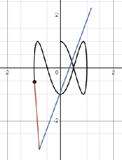
has the initial condition\displaystyle \left( {a,F(a))} \right), then the solution is\displaystyle F\left( x \right)=F\left( a \right)+\int_{a}^{x}{{f\left( x \right)dx}}. Solution may also be subject to domain restrictions

Topic 7.8 Exponential Models with Differential Equations Applications include linear motion and exponential growth and decay. The growth and decay model is \displaystyle \frac{{dy}}{{dt}}=kt with the initial condition \displaystyle \left( {0,y\left( 0 \right)} \right) has the solution \displaystyle y=y\left( 0 \right){{e}^{{kt}}}

Topic 7.9 Logistic Models with Differential Equations (BC ONLY) The model of logistic growth, \displaystyle \frac{{dy}}{{dx}}=ky\left( {a-y} \right), can be solved by separating the variables and using partial fraction decomposition. This has never been tested (probably because solving requires a large amount of complicated algebra). Students are expected to know how to interpret the properties of the solution directly from the differential equation (asymptotes, carrying capacity, point where changing the fastest, etc.) and discuss what they mean in context without actually solving the equation.


Timing

The suggested time for Unit 7 is  8 – 9 classes for AB and 9 – 10 for BC of 40 – 50-minute class periods, this includes time for testing etc.


Previous posts on these topics for both AB and BC include:

Differential Equations  A summary of the terms and techniques of differential equation and the method of separation of variables

Domain of a Differential Equation – On domain restrictions.

Accumulation and Differential Equations 

Slope Fields

An Exploration in Differential Equations An exploration illustrating many of the ideas of differential equations. The exploration is here in PDF form and the solution is here. The ideas include: finding the general solution of the differential equation by separating the variables, checking the solution by substitution, using a graphing utility to explore the solutions for all values of the constant of integration, finding the solutions’ horizontal and vertical asymptotes, finding several particular solutions, finding the domains of the particular solutions, finding the extreme value of all solutions in terms of C, finding the second derivative (implicit differentiation), considering concavity, and investigating a special case or two. 

Posts on BC Only Topics

Euler’s Method

Euler’s Method for Making Money

The Logistic Equation 

Logistic Growth – Real and Simulated

Adapting 2021 AB 6

Adapting 2021 BC 5