A recent thread on the AP Calculus Community bulletin boards concerned polar equations. One teacher observed that her students do not have a very solid understanding of polar graphs when they get to calculus. I expect this is a common problem. While ideally the polar coordinate system should be a major topic in pre-calculus courses, this is sometimes not the case. Some classes may even omit the topic entirely. Getting accustomed to a new coordinate scheme and a different way of graphing is a challenge. I remember not having that good an understanding myself when I entered college (where first-year calculus was a sophomore course). Seeing an animated version much later helped a lot.
This blog post will discuss the basics of polar equations and their graphs. It will not be as much as students should understand, but I hope the basics discussed here will be a help. There are also some suggestions for extending the study of polar function as the end.
Instead of using the Cartesian approach of giving every point in the plane a “name” by giving its distance from the y-axis and the x-axis as an ordered pair (x,y), polar coordinates name the point differently. Polar coordinates use the ordered pair (r, θ), where r, gives the distance of the point from the pole (the origin) as a function of θ, the angle that the ray from the pole (origin) to the point makes with the polar axis, (the positive half of the x-axis).
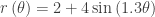
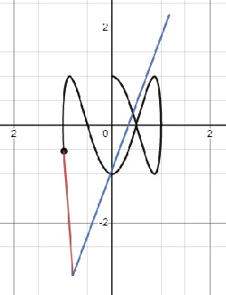
Start with this Desmos graph. It will help if you open it and follow along with the discussion below. The equation in the example is  You may change this to explore other graphs. (Because of the way Desmos graphs, you cannot have a slider for θ; the a-slider will move the line and the point on the graph. r(a) gives the value of r(θ).
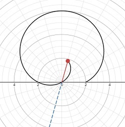
- Notice that as the angle changes the point at varying distance from the pole traces a curve.
- Move the slider to π/6. Since sin(π/6) = 0.5, r(π/6) = 4. The red dot is at the point (4, π/6). Move the slider to other points to see how they work. For example, θ = π/2 gives the point (6,π/2).
- When the slider gets to θ = 7π/6, r = 0 and the point is at the pole. After this the values of r are negative, and the point is now on the ray opposite to the ray pointing into the third and fourth quadrants. The dashed line turns red to remind you of this.
- As we continue around, the point returns to the origin at θ = 11π/6, then values are again positive.
- The graph returns to its starting point when θ = 2π. Note (2,0) is the same point as (2, 2π).
- Even though this is the graph of a function, some points may be graphed more than once and the vertical line test does not apply.
- If we continued around, the graph will retrace the same path. This often happens when the polar function contains trig functions with integer multiples of θ.
- This does not usually happen if no trig functions are involved – try the spiral r = θ.
- If you enter non-integer multiples of θ and extend the domain to large values, vastly different graphs will appear, often making nice designs. Try
 for
for  . This is an area for exploration (if you have time).
In pre-calculus courses several families of polar graphs are often studied and named. For example, there are cardioids, rose curves, spirals, limaçons, etc. The AP Exams do not refer to these names and students are not required to know the names. The exception is circles which have the following forms where R is the radius: θ=R, r = Rsin(θ) or r = Rsin(θ)
To change from polar to rectangular for use the equations  and
and  . This is simple right triangle trigonometry (draw a perpendicular from the point to the x-axis and from there to the pole).
To change from rectangular to polar form use  and
and 
AP Calculus Applications
There are two applications that are listed on the AP Calculus Course and Exam Description: using and interpreting the derivative of polar curves (Unit 9.7) and finding the area enclosed by a polar curve(s) (Units 9.8 and 9.9).
Since calculus is concerned with motion, AP Students should be able to analyze polar curves for how things are changing:
- The rate of change of r away from or towards the pole is given by

- The rate of change of the point with respect to the x-direction is given by
 where
where  from above.
 - The rate of change of the point with respect to the y-direction is given by
 where
where  from above.
 - The slope of the tangent line at a point on the curve is
 . See 2018 BC5 (b)
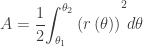
Area

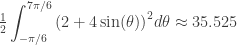
CAUTION: In using this formula, we need to be careful that the curve does not overlap itself. In the Desmos example, the smaller loop overlaps the larger loop; integrating from 0 to 2π counts the inner loop twice. Notice how this is handled by considering the limits of integration dividing the region into non-overlapping regions:
- The area of the outer loop is
- The area of the inner loop is
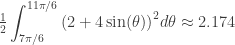
- Integrating over the entire domain gives the sum of these two:
 . This is not the correct area of either part.
This problem can be avoided by considering the geometry before setting up the integral: make sure the areas do not overlap. Restricting r to only non-negative values is often required by the fine print of the theorem in textbooks, but this restriction is not necessary when finding areas and makes it difficult to find, say, the area of the smaller inner loop of the example. Here is another example:
 . Between 0 and
  this curve traces the same path twice.


 . As you rotate the ray you can see the polar graph drawn. When
  the segment extend in the opposite direction from the ray.
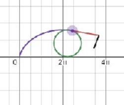
 , on the interior of the wheel (
 ), or outside the wheel (
 – think the flange on a train wheel). Use the “u” slider to animate the drawing. The velocity and acceleration vectors are shown; they may be turned off. The velocity vector is tangent to the curve (not to the circle) and seems to “pull” the point along the curve. The acceleration vector “pulls” the velocity vector. The equation in this demo should not be changed.
 to convert from polar to parametric form,
 since
since 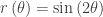 , shown below, appears to show 4 maximums. However, if we trace the graph, we find that these points are (1, π/4), (–1, 3π/4), (1, 5π/4) and (–1, 7π/4). Two of the values are maximums where r(θ) = 1 and two are minimums where r(θ) = –1.
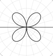

 The domain is extended to