
Now that you know how to compute derivatives it is time to use them. The next few topics and my next few posts will discuss some of the applications of derivatives, and some of the things you can use them for.
The first is linear motion or motion along a straight line.
Derivatives give the rate of change of something that is changing. Linear motion problems concern the change in the position of something moving in a straight line. It may be someone riding a bike, driving a car, swimming, or walking or just a “particle” moving on a number line.
The function gives the position of whatever is moving as a function of time. This position is the distance from a known point often the origin. The time is the time the object is at the point. The units are distance units like feet, meters, or miles.
The derivative position is velocity, the rate of change of position with respect to time. Velocity is a vector; it has both magnitude and direction. While the derivative appears to be just a number its sign counts: a positive velocity indicates movement to the right or up, and negative to the left or down. Units are things like miles per hour, meters per second, etc.
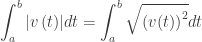
The absolute value of velocity is the speed which has the same units as velocity but no direction.
The second derivative of position is acceleration. This is the rate of change of velocity. Acceleration is also a vector whose sign indicates how the velocity is changing (increasing or decreasing). The units are feet per minute per minute or meters per second per second. Units are often given as meters per second squared (m/s2) which is correct but meters per second per second helps you understand that the velocity in meters per second is changing so much per second.
Of these four, velocity may be the most useful. You will learn how to use the velocity (the first derivative) and its graph to determine how the particle moves over intervals of time: when it is moving left or right, when it stops, when it changes direction, whether it is speeding up or slowing down, how far the object moves, and so on. You can also find the position from the velocity if you also know the starting position.
You will work with equations and with graphs without equations. Reading the graphs of velocity and acceleration is an important skill to learn.
The reasoning used in linear motion problems is the same as in other applications. What you do is the same; what it means depends on the context.
Not to scare anyone, but linear motion problems appear as one of the six free-response questions on the AP Calculus exams almost every year as well as in several the multiple-choice questions.
So, let’s get moving!
Course and Exam Description Unit 4 Sections 4.1 and 4.2
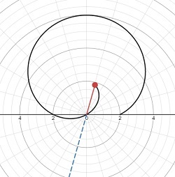
 , in radians between the ray and the polar axis. On the ray is a segment with a point at its end. This segment’s length is
  . As you rotate the ray you can see the polar graph drawn. When
  the segment extend in the opposite direction from the ray.
 , for example
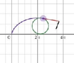
 , on the interior of the wheel (
 ), or outside the wheel (
 – think the flange on a train wheel). Use the “u” slider to animate the drawing. The velocity and acceleration vectors are shown; they may be turned off. The velocity vector is tangent to the curve (not to the circle) and seems to “pull” the point along the curve. The acceleration vector “pulls” the velocity vector. The equation in this demo should not be changed.
 notation for vectors. Any of the usual notations may be used by students, but be sure to show them the others in case the one their book usage is different than the exam’s.)

 , this is the same formula reduced to one dimension.


 . Velocity is has direction (indicated by its sign) and magnitude. Technically, velocity is a vector; the term “vector” will not appear on the AB exam.
 . It, too, has direction and magnitude and is a vector.
 .
. . Note that “displacement” has not been used preciously on AP exam, but (as per the new Course and Exam Description) may be used now. Be sure your students know this term.
 Notice that this is an accumulation function equation (Type 1).
 .
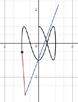
. (blue graph) of a particle moving on the interval
  . The red graph is
  are reflected over the x-axis. (The graphs overlap on [b, d].) It is now quite east to see that the speed is increasing on the intervals [0,a], [b, c] and [d,e].

