Motion Problems: Same Thing, Different Context

Posted on October 8, 2021 by Lin McMullin

Calculus is about things that are changing. Certainly, things that move are changing, changing their position, velocity, and acceleration. Most calculus textbooks deal with things being dropped or thrown up into the air. This is called uniformly accelerated motion since the acceleration is due to gravity and is constant. While this is a good place to start, the problems are by their nature somewhat limited. Students often know all about uniformly accelerated motion from their physics class.

The Advanced Placement exams take motion problems to a new level. AB students often encounter particles moving along the x-axis or the y-axis (i.e. on a number line) according to a function that gives the particle’s position, velocity, or acceleration. BC students often encounter particles moving around the plane with their coordinates given by parametric equations or their velocity given by a vector. Other times the information is given as a graph or even in a table of the position or velocity. The “particle” may become a car, or a rocket or even chief readers riding bicycles.

While these situations may not be all that “real”, they provide excellent ways to ask both differentiation and integration questions. but be aware that they are not covered that much in some textbooks; supplementing the text may be necessary.

The main derivative ideas are that velocity is the first derivative of the position function, acceleration is the second derivative of the position function and the first derivative of the velocity. Speed is the absolute value of velocity. (There will be more about speed in the next post.) The same techniques used to find the features of a graph can be applied to motion problems to determine things about the moving particle.

So, the ideas are not new, but the vocabulary is. The table below gives the terms used with graph analysis and the corresponding terms used in motion problem.

Vocabulary: Working with motion equations (position, velocity, acceleration) you really do all the same things as with regular functions and their derivatives. Help students see that while the vocabulary is different, the concepts are the same.

Function Linear Motion
Value of a function at x position at time t
First derivative velocity
Second derivative acceleration
Increasing moving to the right or up
Decreasing moving to the left or down
Absolute Maximum farthest right
Absolute Minimum farthest left
yʹ = 0 “at rest”
yʹ changes sign object changes direction
Increasing & cc up speed is increasing
Increasing & cc down speed is decreasing
Decreasing & cc up speed is decreasing
Decreasing & cc down speed is increasing
Speed absolute value of velocity

Here is a short quiz on this idea.

Revised and updated from a post originally published on November 16, 2012

Unit 4 – Contextual Applications of the Derivative

Posted on October 5, 2021 by Lin McMullin

Unit 4 covers rates of change in motion problems and other contexts, related rate problems, linear approximation, and L’Hospital’s Rule. (CED – 2019 p. 82 – 90). These topics account for about 10 – 15% of questions on the AB exam and 6 – 9% of the BC questions.

You may want to consider teaching Unit 5 (Analytical Applications of Differentiation) before Unit 4. Notes on Unit 5 will be posted next Tuesday September 29, 2020

Topics 4.1 – 4.6

Topic 4.1 Interpreting the Meaning of the Derivative in Context Students learn the meaning of the derivative in situations involving rates of change.

Topic 4.2 Linear Motion The connections between position, velocity, speed, and acceleration. This topic may work better after the graphing problems in Unit 5, since many of the ideas are the same. See Motion Problems: Same Thing, Different Context

Topic 4.3 Rates of Change in Contexts Other Than Motion Other applications

Topic 4.4 Introduction to Related Rates Using the Chain Rule

Topic 4.5 Solving Related Rate Problems

Topic 4.6 Approximating Values of a Function Using Local Linearity and Linearization The tangent line approximation

Topic 4.7 Using L’Hospital’s Rule for Determining Limits of Indeterminate Forms. Indeterminate Forms of the type $\displaystyle \tfrac{0}{0}$ and $\displaystyle \tfrac{{\pm \infty }}{{\pm \infty }}$ . (Other forms may be included, but only these two are tested on the AP exams.)

Topic 4.1 and 4.3 are included in the other topics, topic 4.2 may take a few days, Topics 4.4 – 4.5 are challenging for many students and may take 4 – 5 classes, 4.6 and 4.7 two classes each. The suggested time is 10 -11 classes for AB and 6 -7 for BC. of 40 – 50-minute class periods, this includes time for testing etc.

This is a re-post and update of the third in a series of posts from last year. It contains links to posts on this blog about the differentiation of composite, implicit, and inverse functions for your reference in planning. Other updated post on the 2019 CED will come throughout the year, hopefully, a few weeks before you get to the topic.

Posts on these topics include:

Motion Problems

Motion Problems: Same Thing, Different Context

Speed

A Note on Speed

Adapting 2021 AB 2

Adapting 2021 AB 4 / BC 4

Related Rates

Adapting 2021 AB 2

Posted on June 29, 2021 by Lin McMullin

Two of nine. Continuing the series started in my last post, this post looks at the AB Calculus 2021 exam question AB 2. The series looks at each question with the aim of showing ways to use the question in with your class as is or by adapting and expanding it. Like most of the AP Exam questions there is a lot more you can ask from the stem and a lot of other calculus you can discuss.

2021 AB 2

This is a Linear Motion Problem (Type 2) and has topics from Unit 4 of the current Course and Exam Description. Two particles are moving on the x-axis and the questions ask about their motion individually and relative to each other. The velocity and initial position are given for each particle. Parts (a), (c), and (d) are typical; (b) is the core of the problem.

The stem is:

Part (a): Students are asked to find the position of each particle at time t = 1.

Discussion and ideas for adapting this question:

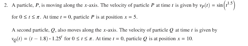
The expected approach is to calculate for each particle the initial position plus the displacement from t = 0 to t = 1. So, for P the computation is $P\left( 1 \right)=5+\int_{0}^{1}{{\sin \left( {{{t}^{{1.5}}}} \right)}}dt$ and similarly for Q(1). This is a calculator allowed question and students should use their calculator to find the answer and not do it by hand.
A different approach is to work it as an initial value differential equation problem. This will work but takes longer than the approach suggested above.
In class, it is worth discussing both methods.
You can adapt this by using a different time.
Another question is to find (only) the displacement if each particle over some time interval. Displacement has been asked in other years.
Ask “Will the particles ever collide? If so when and justify your answer. (Answer: no)

Part (b): Students were asked to determine if the particles are moving apart or towards each other at time t = 1. This is the main question and requires a careful analysis of their motion.

Discussion and ideas for adapting this question:

To determine this, students need to consider the velocity of the particles and their position (from part (a)). P is to the left of Q and moving right. Q is to the right of P and moving left, therefore, the distance between them is decreasing.
You can practice this analysis by using different times.
Ask students to carefully describe the motion of one or both particles: when it is moving left and right, when it changes direction, find the local maximum and minimum positions, etc. Notice that this is really the same as analyzing the shape of a graph. The connection between the two problems will help students understand both better. See: Motion Problems: Same Thing, Different Context

Part (c): A question about speed.

Discussion and ideas for adapting this question:

A typical question. Students should compare the signs of the velocity and acceleration of the particle. If they are the same, the speed is increasing; if different, decreasing.
You may ask this of the other particle.
You may ask this at different times.
See previous posts on speed here and here.

Part (d): Students were required to find the total distanced traveled by Q on the interval [0, π].

Discussion and ideas for adapting this question:

Since speed is the absolute value of the velocity, integrate the absolute value of the velocity. Do this on a calculator.
Adapt this by using a different interval.
Adapt this by using the other particle.
Another (longer) way to approach this question is to find where the particle changes direction by finding where the velocity changes from negative to positive and/or vice versa (i.e., the local extreme values). Then find the distanced traveled on each part of the “trip,” and add or subtract. This will reinforce a lot of the concepts involved in linear motion; that is why it is worth doing. As for the exam, integrating the absolute value is the way to go. However, if this were a non-calculator question, then it would have to be done this way. Find a simpler velocity and try it both ways.
To integrate the absolute value by hand, it is necessary to break the interval into subintervals depending on where the velocity is positive or negative. This is the same as the approach in the bullet immediately above. This, too, is worth showing to reinforce the definition of absolute value.

2021 revised as an in-out question.

There was some unhappiness over the fact that the 2021 AB Calculus exam did not have an in-out questions (Rate and Accumulation Type 1). However, this question does have two rates going in opposite directions. So, just to be ornery, I rewrote it as an in-out questions by changing the context and units while keeping the same velocity functions. The point is that the situation tested can be reframed in other ways. Seeing the same thing in different dress may help students concentrate on the calculus involved. Here it is:

A factory processes cement at the rate of $\displaystyle {{v}_{p}}\left( t \right)=\sin \left( {{{t}^{{1.5}}}} \right)$ tons per hour for $\displaystyle 0\le t\le \pi$ hours. At time t = 0 the amount on hand is P = 5 tons.

The factory ships the cement at a rate given by $\displaystyle {{v}_{Q}}\left( t \right)=\left( {t-1.8} \right){{1.25}^{t}}$ tons per hour for $\displaystyle 0\le t\le \pi$ hours. At time t = 0 the amount shipped is 10 tons.

Find the amount processed and the amount shipped after hour.
Is the amount on hand increasing or decreasing at time t = 1? Explain your reasoning.
At what rate is the rate at which the cement is being shipped changing at t = 1? Is the amount being shipped increasing or decreasing at t = 1? Explain your reasoning.
Find the total amount of cement processed over the time interval $\displaystyle 0\le t\le \pi$ .

Next week 2021 AB 3/ BC 3.

I would be happy to hear your ideas for other ways to use this questions. Please use the reply box below to share your ideas.

Contextual Applications of the Derivative – Unit 4

Posted on September 22, 2020 by Lin McMullin

You may want to consider teaching Unit 5 (Analytical Applications of Differentiation) before Unit 4. Notes on Unit 5 will be posted next Tuesday September 29, 2020

Topics 4.1 – 4.6

Topic 4.1 Interpreting the Meaning of the Derivative in Context Students learn the meaning of the derivative in situations involving rates of change.

Topic 4.3 Rates of Change in Contexts Other Than Motion Other applications

Topic 4.4 Introduction to Related Rates Using the Chain Rule

Topic 4.5 Solving Related Rate Problems

Topic 4.6 Approximating Values of a Function Using Local Linearity and Linearization The tangent line approximation

Topic 4.7 Using L’Hospital’s Rule for Determining Limits of Indeterminate Forms. Indeterminate Forms of the type $\displaystyle \tfrac{0}{0}$ and $\displaystyle \tfrac{\infty }{\infty }$ . (Other forms may be included, but only these two are tested on the AP exams.)

Posts on these topics include:

Motion Problems

Motion Problems: Same Thing, Different Context

Speed

A Note on Speed

Related Rates

2019 CED Unit 4: Contextual Applications of the Derivative

Posted on October 7, 2019 by Lin McMullin

Unit 4 covers rates of change in motion problems and other contexts, related rate problems, linear approximation and L’Hospital’s Rule. (CED – 2019 p. 82 – 90). These topics account for about 10 – 15% of questions on the AB exam and 6 – 9% of the BC questions.

Topics 4.1 – 4.6

Topic 4.1 Interpreting the Meaning of the Derivative in Context Students learn the meaning of the derivative in situations involving rates of change.

Topic 4.3 Rates of Change in Contexts Other Than Motion Other applications

Topic 4.4 Introduction to Related Rates Using the Chain Rule

Topic 4.5 Solving Related Rate Problems

Topic 4.6 Approximating Values of a Function Using Local Linearity and Linearization The tangent line approximation

Topic 4.7 Using L’Hospital’s Rule for Determining Limits of Indeterminate Forms. Indeterminate Forms of the type $\displaystyle \tfrac{0}{0}$ and $\displaystyle \tfrac{\infty }{\infty }$ . (Other forms may be included, but only these two are tested on the AP exams.)

Posts on these topics include:

Motion Problems

Motion Problems: Same Thing, Different Context

Speed

A Note on Speed

Related Rates

Extreme Values and Linear Motion

Posted on October 24, 2017 by Lin McMullin

Two more applications of differentiation are finding extreme values and the analysis of linear motion.

Extreme Values

The Marble and the Vase

Extremes without Calculus

A Standard Problem

Far Out!

Linear Motion – Motion on a Line

Type 2 Problems

Motion Problems: Same Thing, Different Context

The Ubiquitous Particle Motion Problem – a PowerPoint Presentation and its Handout

Brian Leonard’s Particle Motion Game Velocity Game and answers Velocity game Answers

Matching Motion – an activity

Speed

Linear Motion (Type 2)

Posted on March 7, 2017 by Lin McMullin

“A particle (or car, or bicycle) moves on a number line ….”

These questions may give the position equation, the velocity equation or the acceleration equation of something that is moving, along with an initial condition. The questions ask for information about motion of the particle: its direction, when it changes direction, its maximum position in one direction (farthest left or right), its speed, etc.

The particle may be a “particle,” a person, car, a rocket, etc. Particles don’t really move in this way, so the equation or graph should be considered to be a model. The question is a versatile way to test a variety of calculus concepts since the position, velocity, or acceleration may be given as an equation, a graph, or a table; be sure to use examples of all three forms during the review.

Many of the concepts related to motion problems are the same as those related to function and graph analysis (Type 3). Stress the similarities and show students how the same concepts go by different names. For example, finding when a particle is “farthest right” is the same as finding the when a function reaches its “absolute maximum value.” See my post for November 16, 2012 for a list of these corresponding terms.

The position, s(t), is a function of time. The relationships are

The velocity is the derivative of the position, ${s}'\left( t \right)=v\left( t \right)$ . Velocity is has direction (indicated by its sign) and magnitude. Technically, velocity is a vector; the term “vector” will not appear on the AB exam.
Speed is the absolute value of velocity; it is a number, not a vector. See my post for November 19, 2012.
Acceleration is the derivative of velocity and the second derivative of position, $\displaystyle a\left( t \right)={v}'\left( t \right)={{s}'}'\left( t \right)$ . It, too, has direction and magnitude and is a vector.
Velocity is the antiderivative of the acceleration
Position is the antiderivative of velocity.

What students should be able to do:

Understand and use the relationships above.
Distinguish between position at some time and the total distance traveled during the time period.
The total distance traveled is the definite integral of the speed $\displaystyle \int_{a}^{b}{\left| v\left( t \right) \right|}\,dt$ .
The net distance traveled, displacement, is the definite integral of the velocity (rate of change): $\displaystyle \int_{a}^{b}{v\left( t \right)}\,dt$ . Note that “displacement” has not been used preciously on AP exam, but (as per the new Course and Exam Description) may be used now. Be sure your students know this term.
The final position is the initial position plus the definite integral of the rate of change from x= a to x = t: $\displaystyle s\left( t \right)=s\left( a \right)+\int_{a}^{t}{v\left( x \right)}\,dx$ Notice that this is an accumulation function equation (Type 1).
Initial value differential equation problems: given the velocity or acceleration with initial condition(s) find the position or velocity. These are easily handled with the accumulation equation in the bullet above.
Find the speed at a given time. The speed is the absolute value of the velocity.
Find average speed, velocity, or acceleration
Determine if the speed is increasing or decreasing.
If at some time, the velocity and acceleration have the same sign then the speed is increasing.If they have different signs the speed is decreasing.
If the velocity graph is moving away from (towards) the t-axis the speed is increasing (decreasing).
See my post for November 19, 2012.
Use a difference quotient to approximate derivative.
Riemann sum approximations.
Units of measure.
Interpret meaning of a derivative or a definite integral in context of the problem

Shorter questions on this concept appear in the multiple-choice sections. As always, look over as many questions of this kind from past exams as you can find.

For some previous posts on this subject see November 16, 19, 2012, January 21, 2013. There is also a worksheet on speed here and on the Resources pages (click at the top of this page).

The BC topic of motion in a plane, (Type 8: parametric equations and vectors) will be discussed in a later post.

Friday March 10: Graph Analysis (Type 3)

Tuesday March 14: Area and Volume (Type 4)

Friday March 17: Table and Riemann sums (Type 5)

Tuesday Match 21: Differential Equations (Type 6)

Friday March 24: Others (Type 7: related rates, implicit differentiation, etc.)

Teaching Calculus

The pleasure lies not in discovering the truth, but in searching for it.

Tag Archives: motion problems

Motion Problems: Same Thing, Different Context

Adapting 2021 AB 2

2021 AB 2

Extreme Values and Linear Motion

Linear Motion (Type 2)

Share this:

Like this:

Topics 4.1 – 4.6

Share this:

Like this:

2021 AB 2

Share this:

Like this:

Topics 4.1 – 4.6

Share this:

Like this:

Topics 4.1 – 4.6

Share this:

Like this:

Share this:

Like this:

Share this:

Like this: