
Now that you know how to compute derivatives it is time to use them. The next few topics and my next few posts will discuss some of the applications of derivatives, and some of the things you can use them for.
The first is linear motion or motion along a straight line.
Derivatives give the rate of change of something that is changing. Linear motion problems concern the change in the position of something moving in a straight line. It may be someone riding a bike, driving a car, swimming, or walking or just a “particle” moving on a number line.
The function gives the position of whatever is moving as a function of time. This position is the distance from a known point often the origin. The time is the time the object is at the point. The units are distance units like feet, meters, or miles.
The derivative position is velocity, the rate of change of position with respect to time. Velocity is a vector; it has both magnitude and direction. While the derivative appears to be just a number its sign counts: a positive velocity indicates movement to the right or up, and negative to the left or down. Units are things like miles per hour, meters per second, etc.
The absolute value of velocity is the speed which has the same units as velocity but no direction.
The second derivative of position is acceleration. This is the rate of change of velocity. Acceleration is also a vector whose sign indicates how the velocity is changing (increasing or decreasing). The units are feet per minute per minute or meters per second per second. Units are often given as meters per second squared (m/s2) which is correct but meters per second per second helps you understand that the velocity in meters per second is changing so much per second.
Of these four, velocity may be the most useful. You will learn how to use the velocity (the first derivative) and its graph to determine how the particle moves over intervals of time: when it is moving left or right, when it stops, when it changes direction, whether it is speeding up or slowing down, how far the object moves, and so on. You can also find the position from the velocity if you also know the starting position.
You will work with equations and with graphs without equations. Reading the graphs of velocity and acceleration is an important skill to learn.
The reasoning used in linear motion problems is the same as in other applications. What you do is the same; what it means depends on the context.
Not to scare anyone, but linear motion problems appear as one of the six free-response questions on the AP Calculus exams almost every year as well as in several the multiple-choice questions.
So, let’s get moving!
Course and Exam Description Unit 4 Sections 4.1 and 4.2
 where the point is
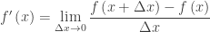
  and the slope is the derivative denoted by
  . You only need these three numbers – the two coordinates of a point and the derivative at that point). Drop them into the point-slope equation and you’re done.)
 million cells per cubic meter
 meters long and whose height is
  meters. This box has a volume of 3
  million plankton in the box.
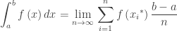
 . Now, if we take thinner boxes by letting
  , we are looking at a Riemann sum. And calculus gives us the answer.
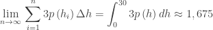 million plankton in the column of water (rounded to the nearest million as directed in the question.)
 . Part (a) asked for the value of
  and also asked students “Using correct units, [to] interpret the meaning of


 million cells per cubic meter. Of course, that thin (thickness
  cells and the cubic meter below has 25.586 million cells. This is a decrease of 1.1767 million cells. So, the derivative is reasonable.
 correct, I included a factor of 1 square meter, this multiplied by p(h) million cells per cubic meter and by dh in meters give a result of millions of cells. More on why this is necessary in Good Question 16 on density.)
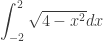 gives the area of a semi-circle of radius 2 feet. The units of the radical are feet and represent the vertical distance from the x-axis to a point in the semi-circle; the dx is the horizontal side of the Riemann sum rectangles also in feet. Both are measured in the same linear units and the area is their product: feet times feet or square feet.