The polynomial function approximates the value of correct to 5 decimal places:
This is not a fluke!
The graph of f(x) is in blue, the sin(x) in red. Note how close the two graphs are in the interval [-2, 2]
Now, approximating the value of a sine function is easier with a calculator. But sines are not the only functions in Math World.
In the Unit 10 you will learn how to write special polynomial functions, called Taylor and Maclaurin polynomials, to approximate any differentiable function you want to as many decimal places as you need. You already know a lot about polynomials. They are easy to understand, evaluate, and graph. The concept of using a polynomial to approximate much more complicated functions is very powerful.
You’ve already got a start on this! Recall that the local linear approximation of a function near x = a is . This is a Taylor Polynomial. And it is the first two terms all the higher degree Taylor polynomial for f near x = a.
To fully understand these polynomials, there is a fair amount of preliminary stuff you need to understand. First you study sequences – functions whose domains are whole numbers. Next comes infinite series. A series is written by adding the terms of a sequence. (Sequences and series may have a finite or infinite number of terms. There is not much to say about finite series; infinite sequences and infinite series are where the action is.) oThe terms 0f some sequences and series are numbers. Other series have powers of an independent variable; these are called power series.
Some power series approximate (converge to) the related function everywhere (i. e. for all Real numbers). Others provide a good approximation only on an interval of finite length. The intervals where the approximation is good is called the interval of convergence. Convergence tests – theorems really – help you determine if a series converges. These in tern help you find the interval of convergence. More on this in my next post.
Depending on your textbook and your teacher, you may study these topics in this order: sequences, convergence test, series, Taylor and Maclaurin polynimials for approximations, and power series. Others may change the order. The path may be different, but the destination will be the same.
Course and Exam Description Unit 10, Sections 10.1, 10.2, 10.11, 10.13, 10.14, 10.15. This is a BC only topic.
Unit 10 covers sequences and series. These are BC only topics (CED – 2019 p. 177 – 197). These topics account for about 17 – 18% of questions on the BC exam.
Topic 10.1: Defining Convergent and Divergent Series.
Topic 10. 2: Working with Geometric Series. Including the formula for the sum of a convergent geometric series.
Topics 10.3 – 10.9 Convergence Tests
The tests listed below are assessed on the BC Calculus exam. Other methods are not tested. However, teachers may include additional methods.
Topics 10.10 – 10.12 Taylor Series and Error Bounds
Topic 10.10: Alternating Series Error Bound.
Topic 10.11: Finding Taylor Polynomial Approximations of a Function.
Topic 10.12: Lagrange Error Bound.
Topics 10.13 – 10.15 Power Series
Topic 10.13: Radius and Interval of Convergence of a Power Series. The Ratio Test is used almost exclusively to find the radius of convergence. Term-by-term differentiation and integration of a power series gives a series with the same center and radius of convergence. The interval may be different at the endpoints.
Topic 10.14: Finding the Taylor and Maclaurin Series of a Function. Students should memorize the Maclaurin series for , sin(x), cos(x), and ex.
Topic 10.15: Representing Functions as Power Series. Finding the power series of a function by differentiation, integration, algebraic processes, substitution, or properties of geometric series.
Timing
The suggested time for Unit 9 is about 17 – 18 BC classes of 40 – 50-minutes, this includes time for testing etc.
Previous posts on these topics:
Before sequences
Amortization Using finite series to find your mortgage payment. (Suitable for pre-calculus as well as calculus)
A Lesson on Sequences. An investigation, which could be used as early as Algebra 1, showing how irrational numbers are the limit of a sequence of approximations. Also, an introduction to the Completeness Axiom.
Eight of nine. We continue our study of the 2021 free-response questions. We will look at ways to adapt, expand, and explore this question to help students better understand it and look at other questions that can be asked based on a similar stem.
2021 BC 5
This is a Differential Equation (Type 6) with a Sequence and Series (Type 10) question included. It contains topics from Units 7 and 10 of the current Course and Exam Description (CED). It is not unusual for AP Calculus exam question to include several of the types in my classification and from several of the units from the CED (here units 7 and 10). In addition, the usual solving an initial value problem and a Euler’s Method approximation are included.
The stem for 2021 BC 5 is:
Part (a): Students were asked to write the second-degree Taylor polynomial for the function centered at x = 1 and then use it to approximate f(2). Students should stop after substituting 2 into their polynomial; no arithmetic or simplification is required, and a simplifying mistake will lose a point.
Discussion and ideas for adapting this question:
Ask students to find an expression for the second derivative (implicit differentiation).
Verify that
Ask students to find the third-degree polynomial and use it to approximate f(2)
Part (b): Students were required to approximate f(2) using Euler’s method with two steps of equal size.
Discussion and ideas for adapting this question:
After you solve the equation in part (c), ask students to compare the approximations from parts (a) and (b) with the exact value. Neither approximation is very close to the exact value. Discuss why this is so. Consider the slope of the graph near x = 2.
Find a more accurate approximation using 3, 4, or more smaller steps. There are graphing calculator programs that will do the arithmetic. Do not hesitate to use them. Students have already shown they know how to do a Euler’s Method approximation; the point is to understand the situation.
Part (c): Finding the solution of the differential equation by separating the variables is expected in this kind of question. The added twist is that the method of integration by parts is necessary to find one of the antiderivatives.
Discussion and ideas for adapting this question:
Be sure not to skip over removing the absolute value signs. The most efficient way is to realize that at (and near) the initial condition y > 0, so |y| = y. What do you do if y < 0?
There is not much you can do differently here. One thing is to change the initial condition. Try a negative value such as f(1) = –4.
As suggested in (b), compare, and discuss the approximations with the exact value.
Next week we will conclude this series of posts with a look at 2021 BC 6.
I would be happy to hear your ideas for other ways to use this question. Please use the reply box below to share your ideas.
Unit 10 covers sequences and series. These are BC only topics (CED – 2019 p. 177 – 197). These topics account for about 17 – 18% of questions on the BC exam.
Topics 10.1 – 10.2
Topic 10.1: Defining Convergent and Divergent Series.
Topic 10. 2: Working with Geometric Series. Including the formula for the sum of a convergent geometric series.
Topics 10.3 – 10.9 Convergence Tests
The tests listed below are tested on the BC Calculus exam. Other methods are not tested. However, teachers may include additional methods.
Topics 10.10 – 10.12 Taylor Series and Error Bounds
Topic 10.10: Alternating Series Error Bound.
Topic 10.11: Finding Taylor Polynomial Approximations of a Function.
Topic 10.12: Lagrange Error Bound.
Topics 10.13 – 10.15 Power Series
Topic 10.13: Radius and Interval of Convergence of a Power Series. The Ratio Test is used almost exclusively to find the radius of convergence. Term-by-term differentiation and integration of a power series gives a series with the same center and radius of convergence. The interval may be different at the endpoints.
Topic 10.14: Finding the Taylor and Maclaurin Series of a Function. Students should memorize the Maclaurin series for , sin(x), cos(x), and ex.
Topic 10.15: Representing Functions as Power Series. Finding the power series of a function by, differentiation, integration, algebraic processes, substitution, or properties of geometric series.
Timing
The suggested time for Unit 9 is about 17 – 18 BC classes of 40 – 50-minutes, this includes time for testing etc.
Previous posts on these topics:
Before sequences
Amortization Using finite series to find your mortgage payment. (Suitable for pre-calculus as well as calculus)
A Lesson on Sequences An investigation, which could be used as early as Algebra 1, showing how irrational numbers are the limit of a sequence of approximations. Also, an introduction to the Completeness Axiom.
A know a lot of people like mathematics because there is only one answer, everything is exact. Alas, that’s not really the case. Numbers written as non-terminating decimals are not “exact;” they must be rounded or truncated somewhere. Even things like and 5/17 may look “exact,” but if you ever had to measure something to those values, you’re back to using decimal approximations.
There are many situations in mathematics where it is necessary to find and use approximations. Two if these that are usually considered in introductory calculus courses are approximating the value of a definite integral using the Trapezoidal Rule and Simpson’s Rule and approximating the value of a function using a Taylor or Maclaurin polynomial.
If you are using an approximation, you need and want to know how good it is; how much it differs from the actual (exact) value. Any good approximation technique comes with a way to do that. The Trapezoidal Rule and Simpson’s Rule both come with expressions for determining how close to the actual value they are. (Trapezoidal approximations, as opposed to the Trapezoidal Rule and Simpson’s Rule per se, are tested on the AP Calculus Exams. The error is not tested.) The error approximation using a Taylor or Maclaurin polynomial is tested on the exams.
The error is defined as the absolute value of the difference between the approximated value and the exact value. Since, if you know the exact value, there is no reason to approximate, finding the exact error is not practical. (And if you could find the exact error, you could use it to find the exact value.) What you can determine is a bound on the error; a way to say that the approximation is at most this far from the actual value. The BC Calculus exams test two ways of doing this, the Alternating Series Error Bound (ASEB) and the Lagrange Error Bound (LEB). These two techniques are discussed in my previous post, Error Bounds. The expressions used below are discussed there.
Examining Some Error Bounds
We will look at an example and the various ways of computing an error bound. The example, which seems to come up this time every year, is to use the third-degree Maclaurin polynomial for sin(x) to approximate sin(0.1).
Using technology to twelve decimal places sin(0.1) = 0.099833416647
The Maclaurin (2n – 1)th-degree polynomial for sin(x) is
So, using the third degree polynomial the approximation is
The error to 12 decimal places is the difference between the approximation and the 12 place value. The error is:
Using the Alternating Series Error Bound:
Since the series meets the hypotheses for the ASEB (alternating, decreasing in absolute value, and the limit of the nth term is zero), the error is less than the first omitted term. Here that is
The actual error is less than B1 as promised.
Using the Legrange Error Bound:
For the Lagrange Error Bound we must make a few choices. Nevertheless, each choice gives an error bound larger than the actual error, as it should.
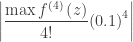
For the third-degree Maclaurin polynomial, the LEB is given by
for some number z between 0 and 0.1.
The fourth derivative of sin(x) is sin(x) and its maximum absolute value between 0 and 0.1 is |sin(0.1)|. So, the error bound is
However, since we’re approximating sin(0.1) we really shouldn’t use it. In a different example, we probably won’t know it.
What to do?
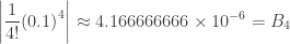
The answer is to replace it with something larger. One choice is to use 0.1 since 0.1 > sin(0.1). This gives
The usual choice for sine and cosine situations is to replace the maximum of the derivative factor with 1 which is the largest value of the sine or cosine.
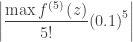
Since the 4th degree term is zero, the third-degree Maclaurin Polynomial is equal to the fourth-degree Maclaurin Polynomial. Therefore, we may use the fifth derivative in the error bound expression, to calculate the error bound. The 5th derivative of the sin(x) is cos(x) and its maximum value in the range is cos(0) =1.
for some number z between 0 and 0.1.
I could go on ….
Since B1, B2, B3, B4, and B5 are all greater than the error, which should we use? Or should we use something else? Which is the “best”?
The error is what the error is. Fooling around with the error bound won’t change that. The error bound only assures you your approximation is, or is not, good enough for what you need it for. If you need more accuracy, you must use more terms, not fiddle with the error bound.


 , sin(x), cos(x), and ex.

 , sin(x), cos(x), and ex
 and 5/17 may look “exact,” but if you ever had to measure something to those values, you’re back to using decimal approximations.
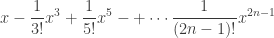


 for some number z between 0 and 0.1.

 to calculate the error bound. The 5th derivative of the sin(x) is cos(x) and its maximum value in the range is cos(0) =1.