Optimization – Reflections

Posted on July 23, 2019 by Lin McMullin

First, a new resource has been added to the resource page. An index of all free-response questions from 1971 – 2018 listed by major topics. These were researched by by Kalpana Kanwar a teacher at Wisconsin Heights High School. Thank you Kalpana! They include precalculus topics that were tested on the exams before 1998. These may be good for your precalculus classes. (Remember that the course description underwent major changes in 1998 and some topics were dropped at that time. These include the “A” topics (precalculus), Newton’s Method, work, volume by cylindrical shells among others. Be careful, when assigning old questions; they’re good, but they may no longer be tested.)

Optimizations problems are situations in which some item is to be made as large or small as possible. Often this is the minimum cost of producing something, or to maximize profit, or to make the largest area or volume with the least material.

While these problems are found in most of the textbooks, they almost never appear on the AP Calculus Exams. The reason for this is that the first step is to write the equation that models the situation. This step does not involve any “calculus.” If a student cannot do this or does it incorrectly, then there is no way to earn the calculus points that follow. On the exams, students are given an expression and asked to find its maximum or minimum value.

Nevertheless, the problems can be interesting and are useful in a practical sense. Reflection is one of my favorites: show that the angle of incidence equals the angle of reflection. In the figure below, light travels from a point A to point D on a reflecting surface CE and then to point B by the shortest total distance. Show that this implies that the angle α between AD and the normal to the surface is equal to the angle β between the normal and DB. The angle α is called the angle of incidence and the angle β is called the angle of reflection.

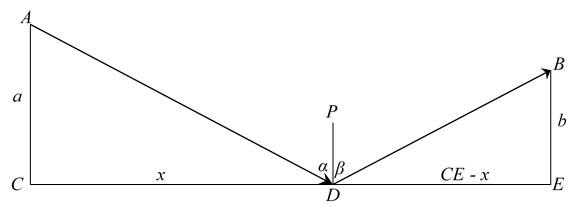
Using the lengths marked in the drawing, $\overline{{AC}},\overline{{PD}}$ and $\overline{{BE}}$ are all perpendicular to $\overline{{CE}}$ the total distance is AD + DB. Therefore:

$AD+DB=\sqrt{{{{a}^{2}}+{{x}^{2}}}}+\sqrt{{{{b}^{2}}+{{{\left( {CE-x} \right)}}^{2}}}}$

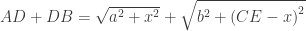
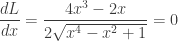
To find the minimum distance find the derivative of AD + DB and set it equal to zero.

$\displaystyle \frac{{2x}}{{2\sqrt{{{{a}^{2}}+{{x}^{2}}}}}}+\frac{{-2\left( {CE-x} \right)}}{{2\sqrt{{{{b}^{2}}+{{{\left( {CE-x} \right)}}^{2}}}}}}=0$

Then

$\displaystyle \frac{x}{{\sqrt{{{{a}^{2}}+{{x}^{2}}}}}}=\frac{{\left( {CE-x} \right)}}{{\sqrt{{{{b}^{2}}+{{{\left( {CE-x} \right)}}^{2}}}}}}$

Now, we need to be clever:

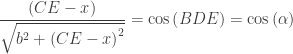
$\displaystyle \frac{x}{{\sqrt{{{{a}^{2}}+{{x}^{2}}}}}}=\cos \left( {ADC} \right)=\cos \left( \beta \right)$ and

$\displaystyle \frac{{\left( {CE-x} \right)}}{{\sqrt{{{{b}^{2}}+{{{\left( {CE-x} \right)}}^{2}}}}}}=\cos \left( {BDE} \right)=\cos \left( \alpha \right)$

And therefore, $\displaystyle \alpha =\beta$ QED.

See the illustration of this in Desmos here and see an easier way to do this problem.

The conic sections all have interesting reflection properties that are quite useful.

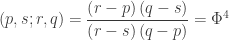
The Ellipse: A light ray leaving one focus of an ellipse is reflected by the ellipse through the other focus of the ellipse. The angle of incidence and the angle of reflection are between the segments to the foci and the normal to the ellipse.

The computation is done using a Computer Algebra System (CAS) and is shown below, the line-byline explanation follows:

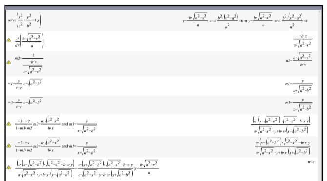
The first line starts with the ellipse $\frac{{{{x}^{2}}}}{{{{a}^{2}}}}+\frac{{{{y}^{2}}}}{{{{b}^{2}}}}=1$ with a > b > 0. Solving for y there are two equations, the second one is for the upper half that we will use below. The other for the lower half.
The second line finds the derivative of y and the third line, m₂ is the slope of the normal, the opposite of the reciprocal of the derivative.
The fourth and fifth lines are the slopes, m₁ and m_3,are the slopes from the point on the ellipse to the foci. The “such that” bar, |, indicates that what follows it is substituted into the expression.
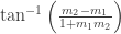
The next two lines compute the inverse tangent of angle rotated counterclockwise between the segments to the foci and the normal. This uses the formula from analytic geometry: ${{\tan }^{{-1}}}\left( {\frac{{{{m}_{2}}-{{m}_{1}}}}{{1+{{m}_{1}}{{m}_{2}}}}} \right)$
The last line shows that the expression from the two lines above it are equal, indicated by the “true” on the right.

An illustration using Desmos is here. Ellipses are used as reflectors in medical and dental equipment so that a relatively dim light source can be concentrated at the place where the doctor or dentist is working without “blinding” everyone in the room. There are also ceilings that reflect sound from one focus to the other without anyone elsewhere in the room hearing. These are only a few of their uses.

The hyperbola: A light ray from one focus of a hyperbola is reflected as though it came from the other focus. This is true whether the reflection is from the side nearer the focus or farther from the focus (reflection from the convex or the concave side.

The computation is like the ellipse computation with only a few sign changes. I will not reproduce it here. If you want to try use $\displaystyle \frac{{{{x}^{2}}}}{{{{a}^{2}}}}-\frac{{{{y}^{2}}}}{{{{b}^{2}}}}=1$ and $c=\sqrt{{{{a}^{2}}+{{b}^{2}}}}$ .

There is a Desmos illustration here. Use the p-slider to move the point. The left side shows the reflection from the “outside” surface; the right side shows the reflection from the “inside” surface.

Hyperbolas are used in telescopes and magnifying mirrors to enlarge the image.

The Parabola: A light ray from the focus is reflected parallel to the axis of symmetry of the parabola Or you can go the other way: light traveling parallel to the axis is reflected to the focus.

If you try to prove this on use $x=a{{y}^{2}}$ to avoid working with an undefined slope. The focus is at $\left( {\frac{a}{4},0} \right)$ .

There is a Desmos illustration here

Parabolic reflectors are used in various kinds of spotlight and telescopes and for radar dishes. They are also used for satellite dishes for cable TV; you may have one at home.

The Marble and the Vase

Posted on October 23, 2014 by Lin McMullin

A fairly common max/min problem asks the student to find the point on the parabola $f\left( x \right)={{x}^{2}}$ that is closest to the point $A\left( 0,1 \right)$ . The solution is not too difficult. The distance, L(x), between A and the point $\left( x,{{x}^{2}} \right)$ on the parabola is given by

$\displaystyle L\left( x \right)=\sqrt{{{\left( x-0 \right)}^{2}}+{{\left( {{x}^{2}}-1 \right)}^{2}}}=\sqrt{{{x}^{4}}-{{x}^{2}}+1}$

And the minimum distance can be found when

$\displaystyle \frac{dL}{dx}=\frac{4{{x}^{3}}-2x}{2\sqrt{{{x}^{4}}-{{x}^{2}}+1}}=0$

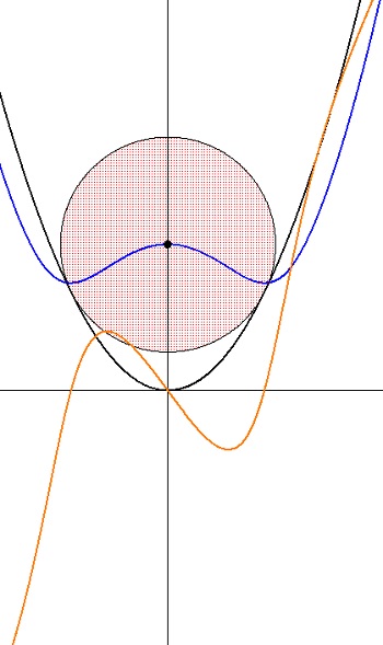
This occurs when $x=0,\frac{1}{\sqrt{2}},-\frac{1}{\sqrt{2}}$ . The local maximum is occurs when x = 0. The (global) minimums are the other two values located symmetrically to the y-axis.

_________________________

Somewhere I saw this problem posed in terms of a marble dropped into a vase shaped like a parabola. So I think of it that way. This accounts for the title of the post. The problem is, however, basically a two-dimensional situation.

In this post I would like to expand and explore this problem. The exploration will, I hope, give students some insight and experience with extreme values, and the relationship between a graph and its derivative. I will pose a series of questions that you could give to your students to explore. I will answer the questions as I go, but you, of course, should not do that until your students have had some time to work on the questions.

Graphing technology and later Computer Algebra Systems (CAS) will come in handy.

_________________________

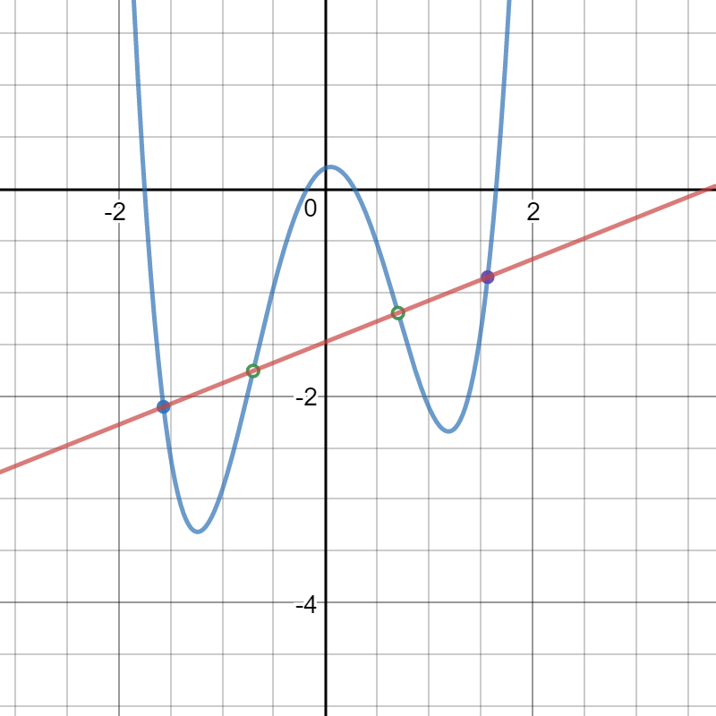
1. Consider a general point $A\left( 0,a \right)$ on the y-axis. Find the x-coordinates of the closest point on the parabola in terms of a.

The distance is now given by

$\displaystyle L\left( x \right)=\sqrt{{{\left( x-0 \right)}^{2}}+{{\left( {{x}^{2}}-a \right)}^{2}}}=\sqrt{{{x}^{4}}+\left( 1-2a \right){{x}^{2}}+{{a}^{2}}}$

$\displaystyle \frac{dL}{dx}=\frac{2{{x}^{3}}+\left( 1-2a \right)x}{\sqrt{{{x}^{4}}+2\left( 1-2a \right){{x}^{2}}+{{a}^{2}}}}$

And $\frac{dL}{dx}=0$ when $x=0,\frac{\sqrt{2\left( 2a-1 \right)}}{2},-\frac{\sqrt{2\left( 2a-1 \right)}}{2}$

The (local) maximum is at x = 0. The other values are the minimums. The CAS computation is shown at the end of the post. This is easy enough to do by hand.

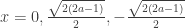
2. Discuss the equation ${{L}^{2}}={{x}^{2}}+{{\left( x-a \right)}^{2}}$ in relation to this situation.

This is the equation of a circle with center at A with radius of L. At the minimum distance this circle will be tangent to the parabola.

3. What happens when $a=\tfrac{1}{2}$ and when $a<\tfrac{1}{2}$ ?

When $a=\tfrac{1}{2}$ , the three zeroes are the same. The circle is tangent to the parabola at the origin and a is the minimum distance.

When $a<\tfrac{1}{2}$ , the circle does not intersect the parabola. Notice that in this case two of the roots of $\frac{dL}{dt}=0$ are not Real numbers.

4. Consider the distance, L(x), from point A to the parabola. As x moves from left to right describe how this length changes. Be specific. Sketch the graph of this distance y = L(x). Where are its (local) maximum and minimum values, relative to the parabola and the circle tangent to the parabola?

The clip below illustrates the situation. The two segments marked L(x) are congruent. The graph of y = L(x) is a“w” shape similar to but not quartic polynomial. The minimums occur directly under the points of tangency of the circle and the parabola. The local maximum is directly over the origin. Is it coincidence that the graph goes through the center of the circle? Explain.

5. Graph $y=\frac{dL}{dx}$ and compare its graph with the graph of $y=L(x)$

L(x) is the blue graph and and L'(x) is the orange graph.
Notice the concavity of L'(x)

6. The graph of $y=\frac{dL}{dx}$ appears be concave up, then down, then (after passing the origin) up, and then down again. There are three points of inflection. Find their x-coordinates in terms of a. How do these points relate to y = L(x) ? (Use a CAS to do the computation)

The points of inflection of the derivative can be found from the second derivative of the derivative (the third derivative of the L(x)). The abscissas are $x=-\sqrt{a},x=0,\text{ and }\sqrt{a}$ . The CAS computation is shown below

CAS Computation for questions 1 and 6.

Apt Apps – 1

Posted on August 7, 2013 by Lin McMullin

I am a very big iPad user. I’m on my third iPad and use it all day. Some days I run the battery from 100% down to 10% without even watching movies or playing music. I have lots of apps, a few of which I have found to be very useful in doing and teaching mathematics. In this post and the next I will share some of my thoughts on those I find most useful.

Disclaimer: I have not used or evaluated all the apps of any of the types discussed here. Nor am I familiar with apps for other tables. These are just the ones I have and like.

Graphing and Computing Apps

By far my favorite grapher is Good Grapher Pro www.graph-calc.com. The app includes a full scientific calculator, solver, 2D grapher (Cartesian, polar, parametric, and implicit) and 3D grapher (Cartesian, cylindrical and spherical). It will graph inequalities in both 2D and 3D. The screenshot below shows some of its versatility.

The graphs are of the functions $\displaystyle y={{2}^{-x}}\sin \left( x \right),\ y={{2}^{-x}}\text{ and }y=-{{2}^{-x}}$ . Note the scales: A domain of about $6\pi$ and a range of only about $\displaystyle 2\times {{10}^{-6}}$ . You can turn on any or all of the extreme values, intersections and intercepts and the points will be marked. Double tap on the screen and you go into trace mode. Tap the color coordinated equation at the top and run your finger along the screen to trace. The current point is shown with circle and the gray vertical line; the coordinates and the derivatives (plural) are in the upper left.

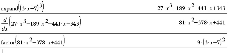
Apps pix 1

The 3D mode is also spectacular. The screen shot show a plane intersecting a cone.

The third screen shot shows the same graph from a different angle clearly showing the hyperbola.

Both the 2D and 3D graphs can have a black or white background. I prefer black, but white is easier to see here. Two improvements would be the ability to graph on a restricted domain and the addition of sliders. The not “pro” version is free but has less functionality.

The TI-Nspire CAS www.education.ti.com is the iPad version of the TI-Nspire CAS calculator. The functionality is the same as the handheld and computer versions. The screen is a huge improvement over the handheld whose screen I find too small and cramped. This has become my choice for CAS work and of course it also has all the calculator, graphing, geometry, spreadsheet, data, statistics and notes features of the handheld and computer versions. In the notes section it even writes properly formatted chemistry expressions.

MyScript Calculator www.VisionObjects.com/en/myscript/math-application/ is a handy app. With it you enter a computation by hand or stylus (i.e. not by typing) and it does the computation (including trig and logarithms, etc.). Very simple and easy. If you enter an equation with one or several question marks in place of the variable it will return the solution in place of the question mark(s).

My Script’s big brother is called Math-Ink. Enter any math object by hand or stylus (i.e. not by typing) and it is copied in symbols at the top of the screen so you can proofread it. Then click the button and it returns the full WolframAlpha results. There is a WolframAlpha app as well, but that requires one-line typed entry. With Math-Ink the results are the same but the entry is much easier.

Of course there are many other apps and more being produced every day. These a re just a few that I am familiar with. Please comment or describe your favorites using the “Leave a Comment” link below.

My next post will show some non-calculator apps that you may find useful in teaching.

Lin McMullin’s Theorem

Posted on July 10, 2013 by Lin McMullin

Mathematics more often tends to delight when it exhibits an unanticipated result rather than conforming to … expectations. In addition, the pleasure derived from mathematics is related in many cases to the surprise felt upon the perception of totally unexpected relationships and unities.

– Mario Livio, The Golden Ratio

I have a theorem named after me. I did not name it, but I did prove it – well more like I tripped over it. It is a calculus related idea. Here is how it came about. I say “came about” because as you will see I did not set out to prove it. I just sort of fell in my lap as I was working on something else.

I was trying to do an animation of an idea that I had heard about: If you have a fourth degree, or quartic, polynomial with a “W” shape it has two points of inflection. If you draw a line through the points of inflection three regions enclosed by the line and the polynomial’s graph are formed. The areas of these regions are in the ratio of 1:2:1. In order to make the animation work I needed the general coordinates of the four points where the line intersects the quartic.

The straightforward way to proceed would be to write a general fourth degree polynomial,

$f\left( x \right)={{c}_{4}}{{x}^{4}}+{{c}_{3}}{{x}^{3}}+{{c}_{2}}{{x}^{2}}+{{c}_{1}}x+{{c}_{0}}$

differentiate it twice to find the second derivative. Then find the zeros of the second derivative (by the quadratic formula), write the equation of the line through them, and then find where else the line intersects the quartic. Without even starting I realized that even with a CAS the algebra and equation solving was going to be really fun (Not!). So, I decided on an alternative approach.

I decided to let the zeros of the second derivative be x = a and x = b, then at least they would be easy to work with. Then the second derivative is $\displaystyle {{f}'}'\left( x \right)=12{{c}_{4}}\left( x-a \right)\left( x-b \right)$ where the ${{c}_{4}}$ is the leading coefficient of the quartic and the 12 comes from differentiating twice.

I integrated to get the first derivative and added ${{c}_{1}}$ , the coefficient of the linear term, as the constant of integration. I integrated again and added ${{c}_{0}}$ , the constant term. as the constant of integration. This resulted in the original quartic function:

$\displaystyle f\left( x \right)={{c}_{4}}{{x}^{4}}-2\left( a+b \right){{c}_{4}}{{x}^{3}}+6ab{{c}_{4}}{{x}^{2}}+{{c}_{1}}x+{{c}_{0}}$

Then I wrote the equation of y(x) the line through the points of inflection. It is too long to copy, but you may see it in the screen capture at the end of the post. (That is what is nice about a CAS: you really do not have to worry about how complicated things are.)

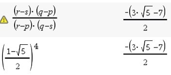
Then I solved the equation $f\left( x \right)=y\left( x \right)$ . Two of the solutions are x = a and x = b as I expected. (This means that you could do synthetic division by hand since you know two of the roots.) The other two I did not expect. They are:

$\displaystyle {{x}_{1}}=\frac{1+\sqrt{5}}{2}a+\frac{1-\sqrt{5}}{2}b$ and $\displaystyle {{x}_{2}}=\frac{1+\sqrt{5}}{2}b+\frac{1-\sqrt{5}}{2}a$

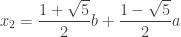
And that’s when I stopped astonished! Those numbers are the Golden Ratio $\Phi =\frac{1+\sqrt{5}}{2}$ , and its reciprocal $\phi ={{\Phi }^{-1}}=\frac{1-\sqrt{5}}{2}$ . So the roots are $\Phi a+\phi b$ and $\Phi b+\phi a$ . How did they get there?

To this day I have no idea why the Golden Ratio should be so involved with quartic polynomials, but there they are in every quartic!

There were no assumptions made about a and b – they could be Complex numbers. In that case there are no points of inflection, but the “line” and the quartic still will have the same value at the four points.

October 16, 2022 Update: If the solutions of $\displaystyle {y}''=0$ are the Complex conjugates $\displaystyle a=\alpha +\beta i$ and $\displaystyle b=\alpha -\beta i$ then $\displaystyle {{x}_{1}}=\alpha +\sqrt{5}\beta i$ and $\displaystyle {{x}_{2}}=\alpha -\sqrt{5}\beta i$ . When graphed on an Argand diagram the four points are collinear on the vertical line at $\displaystyle x=\alpha$

This was all in 2013 and until just this year I never checked the ratio of the areas. (They check.)

Here is a CAS printout of the entire computation.

An interactive Desmos demo of this can be found here

October 16, 2022, Update: If the solutions of $\displaystyle {y}''=0$ are the Complex conjugates $\displaystyle a=\alpha +\beta i$ and $\displaystyle b=\alpha -\beta i$ then $\displaystyle {{x}_{1}}=\alpha +\sqrt{5}\beta i$ and $\displaystyle {{x}_{2}}=\alpha -\sqrt{5}\beta i$ . When graphed on an Argand diagram the four points are collinear on the vertical line at $\displaystyle x=\alpha$

November 10, 2020, Update: I received an email this week form Dominique Laurain, a computer science and applied math engineer from France, who describes himself as a mathematics hobbyist. He discovered another interesting relationship between the coordinates of the x-coordinates of the four points on the line described above. The four points on the line through the points of inflection of a fourth degree polynomial with Real roots in the drawing above from left to right are p, q, r, and s. The coordinates of the points of inflection are a and b as in the post above.

One, of several, cross-ratios of four points with x-coordinates of p, q r, and s is defined as

$\displaystyle (p,s;r,q)=\frac{{\left( {r-p} \right)\left( {q-s} \right)}}{{\left( {r-s} \right)\left( {q-p} \right)}}$ .

Dominique Laurin discovered that $\displaystyle (p,s;r,q)=\frac{{\left( {r-p} \right)\left( {q-s} \right)}}{{\left( {r-s} \right)\left( {q-p} \right)}}={{\Phi }^{4}}$

The computation is shown in the figure below.

There are 24 other cross-ratios depending on the order of the points. In groups of 4, the 24 possible orders are equal to 6 related values. See the cross-ratio link above above. For example, the cross-ratio in the order (s, p; r, q) is ${{\varphi }^{4}}$

Also, $(q,r;s,p)={{\Phi }^{4}}$

Other interesting information:

The Golden Ratio also appears in cubic equations. See the Tashappat – McMullin theorem here.

“Quartic Polynomials and the Golden Ratio” by Harald Totland of the Royal Norwegian Naval Academy. (June 2009)

Speaking of the Golden Ratio, the Calculus Humor website has a nice feature on the Golden Ratio in logos. To view it click here.

Link for cross-ratios

Revised and updated July 20 and 23, 2017, November 10, 2020

Experimenting with CAS – Chain Rule

Posted on July 3, 2013 by Lin McMullin

Discovering things in mathematics can be facilitated by using a computer algebra system (CAS) available on many handheld calculators and computer apps. A CAS can provide good data with which to draw conclusions. You can do “experiments” by producing the results with a CAS and looking for patterns. As an example, let’s look at how you and your students might discover the chain rule for derivatives.

One of the ways you could introduce the chain rule is to ask your class to differentiate something like (3x + 7)². Not knowing about the chain rule, just about the only way to proceed is to expand the expression to 9x² + 42x + 49 and differentiate that: 18x + 42 and then factor 6(3x + 7). Then you show how this relates to the power rule and where the “extra” factor of 3 comes from differentiating the (3x + 7). You really cannot a much more complicated example, say a third or fourth power, because the algebra gets complicated very fast.

Or does it?

Suggest your students use a CAS to do the example above this time using the third power. The output might look like this:

But even better: what we want is just the answer. Who cares about all the algebra in between? Try a few powers until the pattern become obvious.

Now we have some good data to work with. Can you guess the pattern?

Nor sure where the “extra” factor of 3 comes from? Try changing the 3 in the original and keep the exponent the same.

Now can you guess the chain rule? See if what you thought is right by changing only the inside exponent.

Then you can try some others:

CAS D

You can count on the CAS giving you the correct data (answers). Do enough experiments until the chain rule pattern becomes clear.

But I think the big thing is not the chain rule, but that the students are learning how to experiment in mathematics situations. In these we started by changing only the outside power. Then we kept the power the same power and changed the coefficient of the linear factor. Then we changed the power inside power, each time seeing if our tentative rule for differentiating composite function was correct and adjusting it if it was not. Finally we tried a variety of different expressions. You change things. Not big things but little things. You don’t jump from one trial to something very different, only something a little different.

You can do the same thing for the product rule, the quotient rule, maybe some integration rules and so on. You have accomplished your goal when the students can produce the data they need without your suggestions.

But be aware: sometimes this can lead to unexpected results. Does the pattern hold here?

Or here?

Hint: $\frac{7}{3.2}=2.1875$ and $3{{\left( 3.2 \right)}^{3}}=98.304$

Revised 8-25-17

Teaching Calculus

The pleasure lies not in discovering the truth, but in searching for it.

Category Archives: CAS

Optimization – Reflections

The Marble and the Vase

Apt Apps – 1

Graphing and Computing Apps

Lin McMullin’s Theorem

Experimenting with CAS – Chain Rule

Share this:

Like this:

Share this:

Like this:

Graphing and Computing Apps

Share this:

Like this:

Share this:

Like this:

Share this:

Like this: