
 Today’s question is not a good question. It’s a bad question.
But sometimes a bad question can become a good one.
This one leads first to a discussion of units, then to all sorts of calculus.
Here’s the question a teacher sent me this week taken from his textbook:
The normal monthly rainfall at the Seattle-Tacoma airport can be approximated by the model
, where R is measured in inches and t is the time in months, t = 1 being January. Use integration to approximate the normal annual rainfall. Hint: Integrate over the interval [0,12].
Of course, with the hint it’s not difficult to know what to do and that makes it less than a good question right there. The answer is 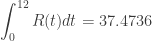
Then a student asked. “If R is in inches shouldn’t be in units of the integral be inch-months, since the unit of an integral is the unit of the integrand times the units of the independent variable?” Well, yes, they should. So, what’s up with that?
Also, the teacher figured that the integral of a rate is an amount and our answer is an amount, so why isn’t the integrand a rate?
The only answer I could come up with is that the statement “R is measured in inches” is incorrect; R should be measured in inches /month. The opening phrase “normal monthly rainfall” also seems to point to the correct units for R being inches/month.
Problem solved; or maybe does this lead to a different concern?
The teacher pointed out that R(6) = 0.7658 inches is a reasonable answer for the amount of rain in June whereas 
If R is a rate, then the amount of rain that falls in June (t = 6) is given by 
From here on we will assume that R is a rate with units of inches/month. Here are the individual monthly rates calculated with a CAS. 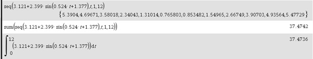
The total amount of rainfall (second line above) appears be R(1) + R(2) + R(3) + … +R(12) = 37.4742. This is very close to the amount calculated by integration.
The slight difference of 0.0006 is not a round off error.
Remember, behind every definite integral there is a Riemann sum!
Again, the units are the problem. Why does the sum of the monthly rates seem to give the total amount? The reason is that the terms of the sequence above are actually the values of a right-side Riemann sum of the rate, R(t), over the interval [0,12] with 12 equal subdivisions of width 1 (month) each with the 1’s left out as 1’s often are. Therefore, their sum should come close to the total yearly rainfall, but it is really just an approximation of it.
The actual total for any month, n, is given by 
Here is the sequence of the actual monthly rainfall values in inches, and their sum.

This agrees with the integral. Why? Because one of the properties of integrals tell us that 
Another instructive thing with this integral is this: The function 

The total rainfall divided by 12 is 

So, there you have it. Is this a good question or not? We considered all these concepts while working not just with an equation but with numbers from a poorly stated problem:
- Reading and interpreting words.
- Unit analysis
- Integration by technology
- Realizing that a pretty good approximation is not correct, due again to units.
- A Riemann sum approximation in a real situation that comes very close to the value by integration
- Using a property of a periodic function to greatly simplify an integral
- Finding average value two ways
So, it turned out to be a sunny day in Seattle.
.

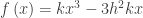 .
. . The leading coefficient k will eventually divide out and not be a concern.
 and
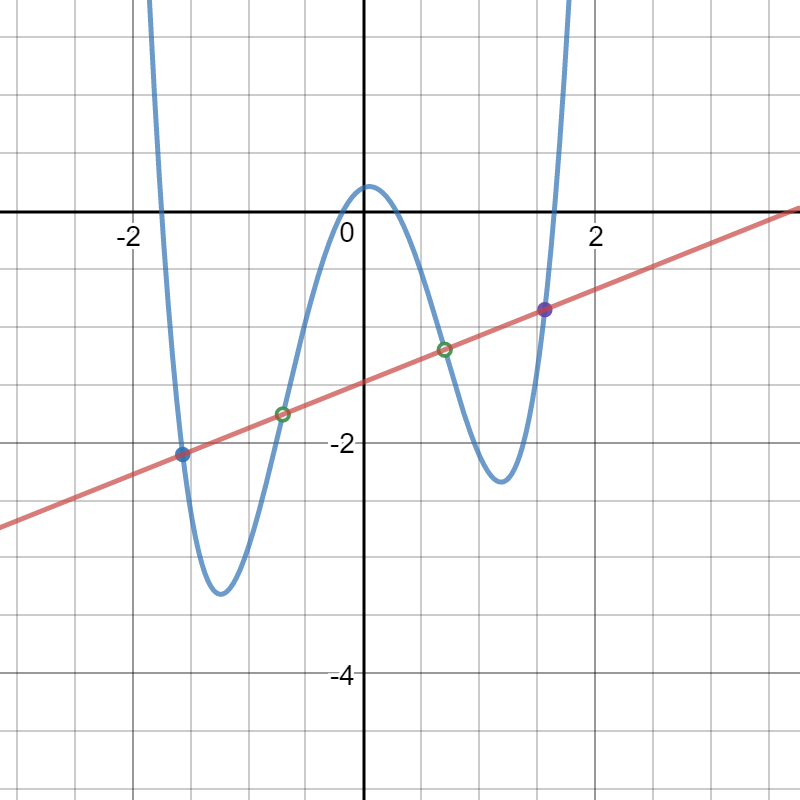
and 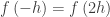 . This means that the extreme values are the same as a point on the graph 3h units away on the other side of the y-axis. This is mildly interesting in itself. The reason it is mentioned id that we will use these points soon.
 which is really true for any points at equal distances on opposite sides of the origin. This is obvious from the symmetry of the cubic.


 . The equation can be solved by hand. We know that x = h is one solution. Synthetic division will give a quadratic and the quadratic formula will do the rest.


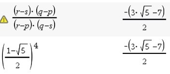
 is the Golden Ratio and
  is the reciprocal of the Golden Ratio.
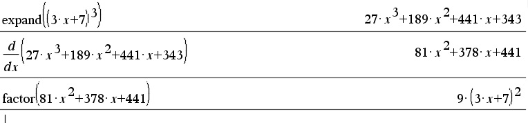
 where the
  is the leading coefficient of the quartic and the 12 comes from differentiating twice.
 , the coefficient of the linear term, as the constant of integration. I integrated again and added
  , the constant term. as the constant of integration. This resulted in the original quartic function:
 . Two of the solutions are x = a and x = b as I expected. (This means that you could do synthetic division by hand since you know two of the roots.) The other two I did not expect. They are:
 and
and 
 , and its reciprocal
  . So the roots are
  and
and  . How did they get there?
 are the Complex conjugates
  and
and  then
then  and
and  . When graphed on an Argand diagram the four points are collinear on the vertical line at

 .
.


 and
and 
