Graphing Taylor Polynomials

Posted on February 7, 2017 by Lin McMullin

The eighth in the Graphing Calculator / Technology series

Here are some hints for graphing Taylor polynomials using technology. (The illustrations are made using a TI-8x calculator. The ideas are the same on other graphing calculators; the syntax may be slightly different.)

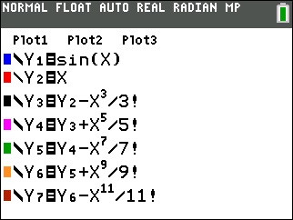
Each successive term of a Taylor polynomial consists of all the previous terms plus one new term. To show students how Taylor polynomials closely approximate a function (in the interval of convergence, of course), enter the function as Y1. Then enter the first term of the polynomial as Y2. Enter the next polynomial as Y3 = Y2 + the second term; enter the next as y4 = Y3 + the next term, and so on.

The example is the McLaurin series for sin(x) centered at the origin:

$\displaystyle \sin \left( x \right)=x-\frac{{{x}^{3}}}{3!}+\frac{{{x}^{5}}}{5!}+\cdots +\frac{{{(-1)}^{2n-1}}{{x}^{2n-1}}}{\left( 2n-1 \right)!}=\sum\limits_{n=1}^{\infty }{{{\left( -1 \right)}^{n+1}}\frac{{{x}^{2n-1}}}{\left( 2n-1 \right)!}}$

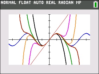
Each will graph one at a time. Watching them graph, one at a time, is instructive as well; each curve approximates the sine curve (in black) further and further away from the origin.

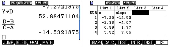
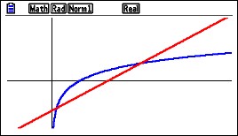
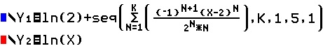
Another way to graph the polynomials is to enter them as a sequence of sums. The example this time is ln(x) centered at x = 2:

$\displaystyle \ln \left( x \right)=\ln \left( 2 \right)+\frac{x-2}{2}-\frac{{{\left( x-2 \right)}^{2}}}{8}+\frac{{{\left( x-2 \right)}^{3}}}{24}+...=\ln \left( 2 \right)+\sum\limits_{n=1}^{\infty }{{{\left( -1 \right)}^{n+1}}\frac{{{\left( x-2 \right)}^{n}}}{{{2}^{n}}n}}$

The syntax is seq( series in sigma notation, indexing variable, start value, end value [,step]). Notice from the figure that the indexing variable, K, is above the sigma.

The individual polynomials graph in the same color (blue); the function is shown in red.

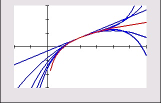Comparing the two graphs (sin(x) and ln(x)) is a good way to start a discussion about the interval of convergence – ask what is different about the graphs as more polynomials are graphed on each. Notice that unlike the sin(x) series the ln(x) polynomials only come close to the function in a limited interval (0, 4) centered at x = 2.

Desmos is also a good program to use to illustrate Taylor and McLaurin polynomials (as are Geogebra and Winplot). The use of the sliders makes it possible to see the successive polynomials quickly. They also help students see the interval of convergence as higher degree polynomials hug the graph on wider intervals (sin(x)), or stay within the same interval (ln(x)). The Desmos illustration with slider for the sin(x) centered at the origin is here and for ln(x) centered at x = 2 is here. Study the input on the left side and enter Taylor polynomials for other functions.

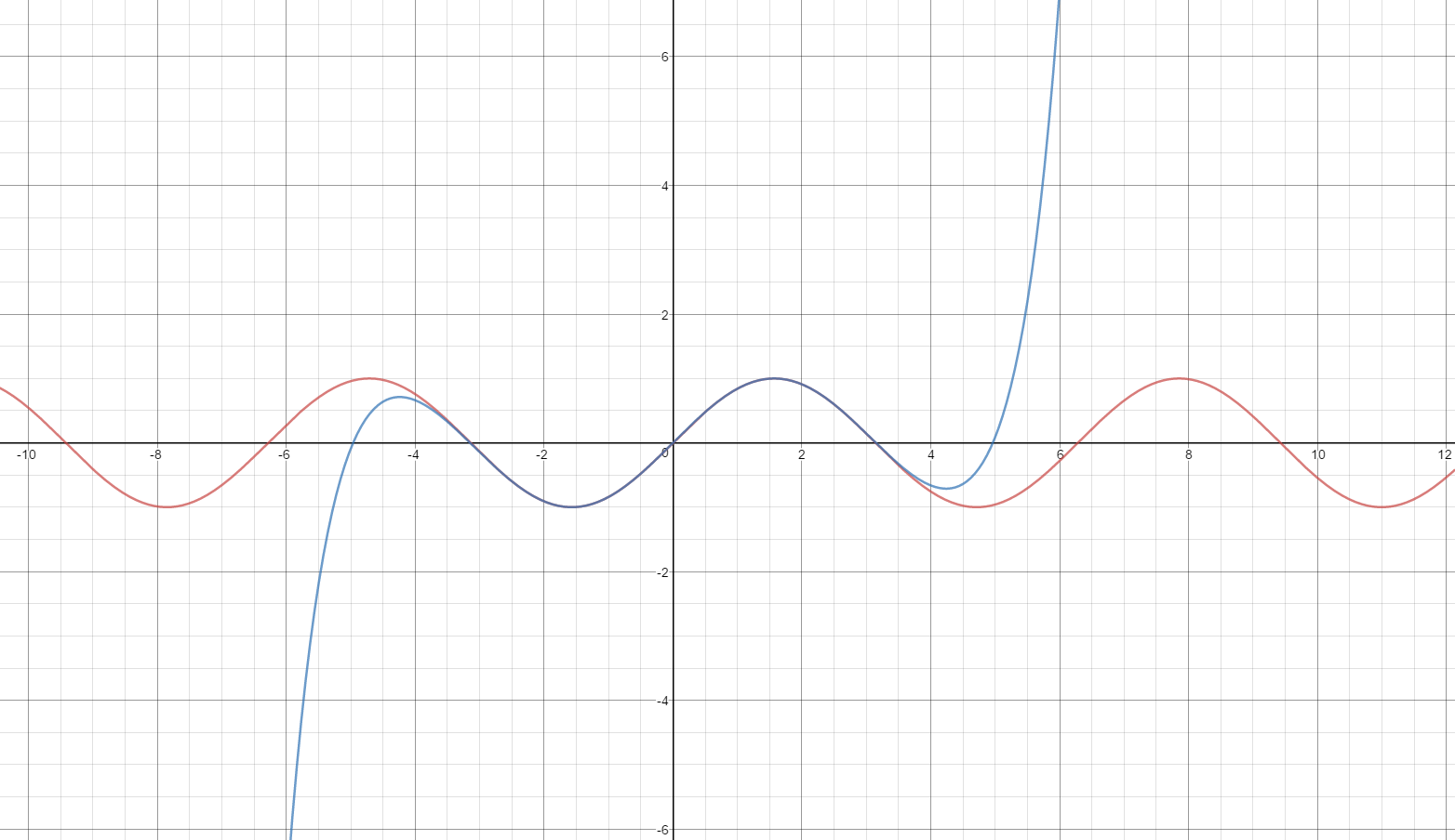
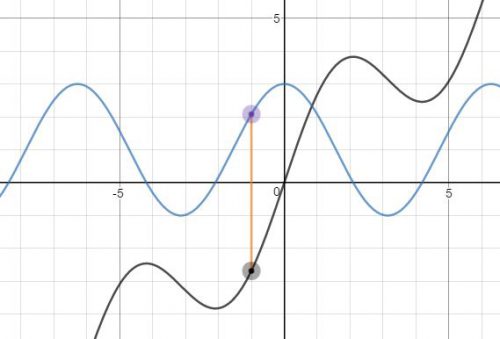
The fifth degree Taylor polynomial for sin(x) centered at the origin.The interval of convergence is all real numbers. Each polynomial “hugs” the graph on wider intervals.

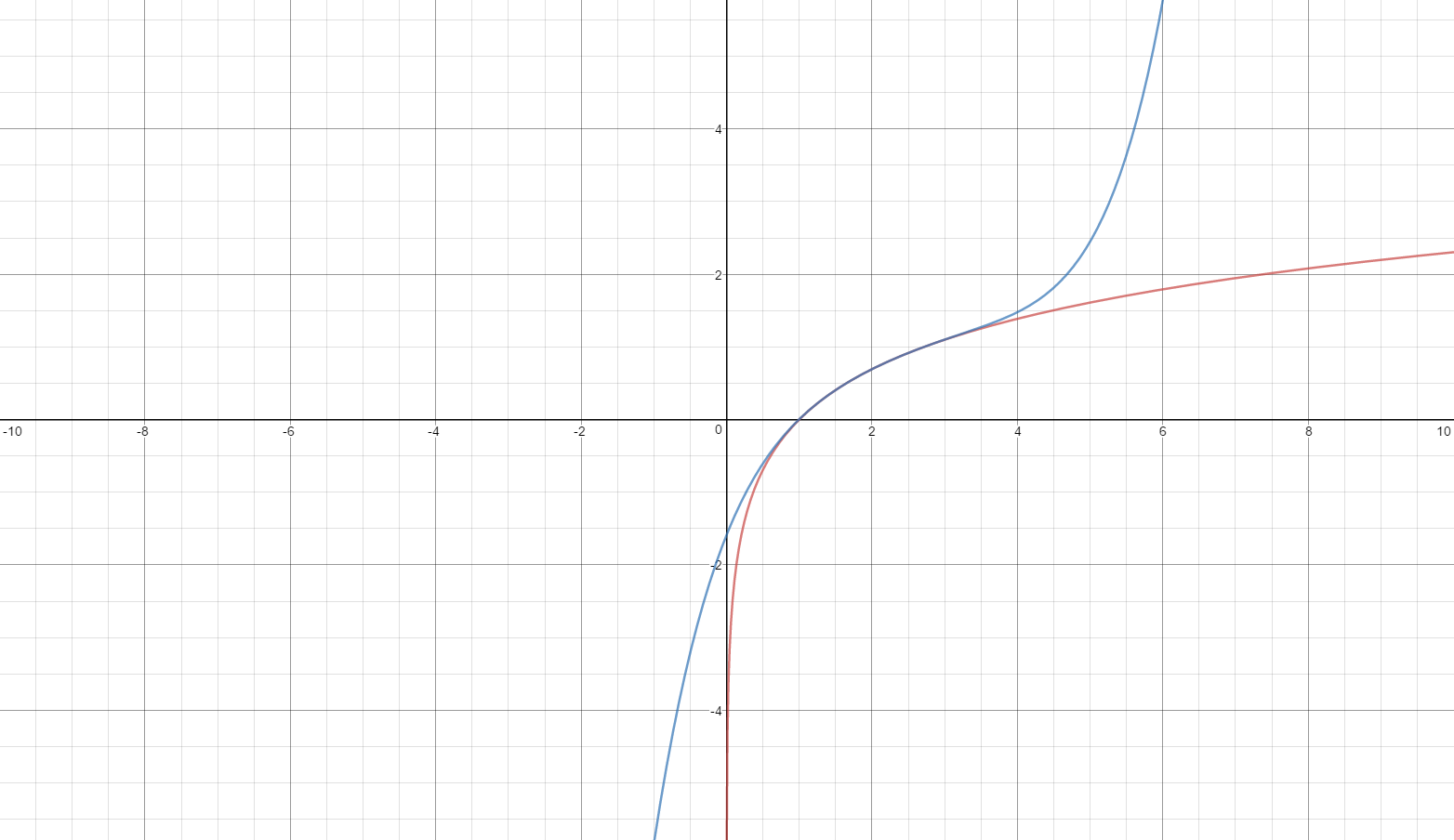
The fifth degree Taylor polynomial for ln(x) centered at x = 2. The interval of convergence is 0 < x < 4. The polynomials all leave the graph outside of this interval.

Coming soon

Feb 14th, Geometric Series – Far Out

Definite integrals – Exam Considerations

Posted on January 3, 2017 by Lin McMullin

The sixth in the Graphing Calculator / Technology Series

Both graphing calculators and CAS calculators allow students to evaluate definite integrals. In the sections of the AP Calculus that allow calculator use students are expected to use their calculator to evaluate definite integrals. On the free-response section, students should write the integral on their paper, including the limits of integration, and then find its value on their calculator. There is no need to show the antiderivative; in fact, the antiderivative may be too difficult to find.

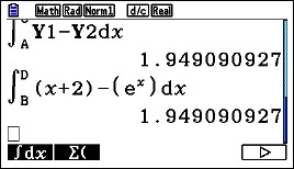
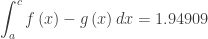
There are a few things students should be aware of. A question typically is worth three points: one point for the limits of integration and any constant (such as $\pi$ in a volume problem), one point for the integrand, and one point for the numerical answer. An answer alone, with no integral, may not earn any points even if it is correct.

The “Instructions” on the cover of the free-response sections read “Show your work. … Your work will be scored on the correctness and completeness of your methods as well as your answers. Answers without supporting work will usually not receive credit.” [Emphasis added] The work must be on the paper, not just on the calculator.

Another consideration is accuracy. The general directions also say, “If you use decimal approximations in calculations, your work will be scored on accuracy. Unless otherwise specified, your final answers should be accurate to three places after the decimal point.”

Let’s see how all this works in an example.

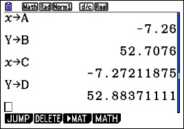
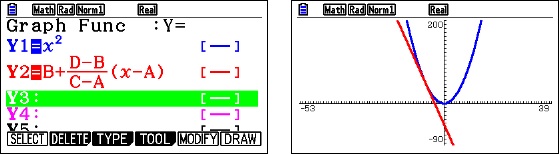
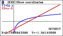
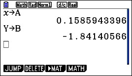
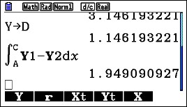
Find the area of the region between the graphs of $f\left( x \right)=x+3\cos (x)$ and $g\left( x \right)={{\left( x-2 \right)}^{2}}$ . Begin by graphing the functions and finding their points of intersections on your graphing calculator.

The values are A = 0.22532 and B = 2.41524 (or 2.41525). Students should also store these values in their calculator and recall them for the computation, as explained in a previous post. Students should write these on their paper just as shown here. Notice that a few extra decimal places should be included. The student should then show the integral and limits along with the answer on their paper:

$\displaystyle \int_{A}^{B}{\left( x-3\cos \left( x \right)-{{\left( x-2 \right)}^{2}} \right)dx=2.32651}$

Notice: Students may write A and B as the limits of integration, provided they have stated their values on the paper. This is best, but they may also write:

$\displaystyle \int_{0.22532}^{2.41525}{\left( x-3\cos \left( x \right)-{{\left( x-2 \right)}^{2}} \right)dx=2.32651}$

or even $\displaystyle \int_{0.225}^{2,415}{\left( x-3\cos \left( x \right)-{{\left( x-2 \right)}^{2}} \right)dx=2.32651}$

But be careful!!! The unrounded values should be used to do the computation. Since the limits are answers they may be rounded, but if the rounding causes the final answer to not be accurate to three places past the decimal point, then the final answer is wrong, and the answer point will not be awarded. This has happened in the past. The safest thing is to use 5 or more decimal places in your computations.

Notice also that the final answer need not be rounded as long as the first three decimal places are correct.

Graphing Integrals

Posted on November 15, 2016 by Lin McMullin

The sixth in the Graphing Calculator / Technology series

The topic of integration is coming up soon. Here are some notes and ideas about the integration operation on graphing calculators. The entries are the same or very similar for all calculator brands.

The basic problem of evaluating a definite integral on a graphing calculator is done without finding an antiderivative; that is, the calculator uses a numerical algorithm to produce the result. The calculator provides a template,and you fill in the 4 squares so that the expression looks exactly like what you write by hand. Then the calculator computes the result. (Older models require a one-line input requiring, in order, the integrand, the independent variable, the lower limit of integration and the upper limit in that order, separated by commas.) The first interesting thing is that the variable in the integrand does to have to be x. As the first figure illustrates using x or a or any other letter gives the same result.

This is because the variable of integration is just a place holder. Sometimes called a “dummy variable”, this letter can be anything at all, including x. On the home or calculation screen you might as well always use x, so the entry will look like what you have on your paper. As we will see, when graphing it may be less confusing to use a different letter.

The antiderivative, F, of any function, f, can be written as a function defined by an integral where there is a point on the antiderivative of f , which is with F ’ = f. The point (a, F(a)) is the initial condition. (In the following we will use F(a) = 0 as the initial condition – the graph will contain the origin. As a further investigation, try changing the lower limit to different numbers and see how that changes the graph.)

The integration operation can be used to graph the antiderivative of a function without finding the antiderivative. You may graph the antiderivative when teaching antiderivatives. Have students look at the graph of the antiderivative and guess what that function is.

When graphing use x as the upper limit of integration and a different letter for the variable in the rest of the template. The calculator will use different values of x to calculate the points to be graphed.

The set-up shown in the next figure shows how to enter a function defined by an integral (blue line) and the same function obtained by antidifferentiating (red squares). As you can see the results are the same.

In this way, you can explore the functions and their indefinite integrals by graphing.

The Fundamental Theorem of Calculus

Another use of using the graph of an integral is to investigate both parts of the Fundamental Theorem of Calculus (FTC). Roughly speaking, the FTC says that the integral of a derivative of a function is that function, and the derivative of an integral is the integrand.

In the figure below, the same function is entered both ways; the graphs are the same. (Note the x’s in the second line must be x in all four places.)

How to Tell your Asymptote from a Hole in the Graph.

Posted on October 4, 2016 by Lin McMullin

The fifth in the Graphing Calculator / Technology series

(The MPAC discussion will continue next week)

Seeing discontinuities on a graphing calculator is possible; but you need to know how a calculator graphs to do it. Here’s the story:

The number you choose for XMIN becomes the x-coordinate of the (center of) the pixels in the left most column of pixels. The number you choose for XMAX is the x-coordinate of the right most column of pixels. The distance between XMIN and XMAX is divided evenly between the remaining pixels so that all the pixels are evenly spaced across the screen (the same distance apart). The rows of pixels are done the same way evenly spacing them between YMIN and YMAX.

This spacing is usually not at “nice” values as can be seen by just moving the cursor across the screen and noticing the x-values or y-values at the bottom of the screen.

The cursor is located one pixel to the right of the y-axis and one pixel above the x-axis in the “standard” window of a TI-8x. Note the coordinates of that pixel at the bottom of the screen. These are the distances between the pixels.

To draw a graph, the calculator takes the x-coordinate of each pixel, calculates the corresponding y-value and turns on the pixel in that column with closest y-pixel-coordinate. If set in a connect mode, the calculator turns on several pixels in adjacent columns so that the y-values seem to connect; this is why the graph often looks jagged in steep sections of the graph. If you are in DOT mode, this does not happen and only one pixel in each column is on.

If you move the cursor over one of the points on a graph, you will see the pixel coordinates, NOT the actual y-coordinates. Use TRACE to see the actual y-coordinate. This is why when finding intersections, you should not just move the cursor over the point, but rather use “intersect” to see the actual y-value of the function.

If the function is undefined for some x-pixel value, then no pixel will turn on in that column. If the function is undefined for some value between the pixel values, then nothing happens because the calculator has not evaluated the function there, so the graph seems to be continuous.

Vertical “asymptotes” are the result of the calculator not evaluating the function at the undefined value; rather it connects the value on one side of the asymptote off the bottom of the screen with the next value on the other side of the asymptote off the top of the screen. If the asymptote appears exactly at a pixel value, then no “asymptote” will appear and that column of pixels will have no pixel turned on. (Some newer calculators and newer operating systems on older calculators have made adjustments so that the “asymptotes” do not show up. In some systems this feature can be turned on or off.)

$The function $latex \displaystyle y=\frac{3\left( x-2 \right)}{\left( x-2 \right)\left( x+2 \right)}$ in the standard window. The vertical line is not really the asymptote and the “hole” at (2, 0.75) is not seen.$

The function $\displaystyle y=\frac{3\left( x-2 \right)}{\left( x-2 \right)\left( x+2 \right)}$ in the standard window. The vertical line is not really the asymptote and the “hole” at (2, 0.75) is not seen.

A removable discontinuity, a hole in the graph (really a skipped pixel), can be seen, if it occurs at a pixel value. Since in most examples the hole is at an integer or other “nice” number, you will not see them in the “standard” window. Use a “decimal” window, which has been chosen in advance so the x-values of the pixels are integers and nice decimals. (To see this, in a decimal window move the cursor around and notice the pixel coordinates).

The other thing you can do is adjust the XMIN and XMAX values so that the distance between them will land on integer values. (Nice project for your class – the number of pixels can be found in the guidebook, or you can count them. In the old days, before decimal windows, this was necessary – it was called finding a “friendly window.”)

$The function $latex \displaystyle y=\frac{3\left( x-2 \right)}{\left( x-2 \right)\left( x+2 \right)}$ in the “decimal” window. The “asymptote” is not shown and the “hole” at (2, 0.75) is visible.$

The function $\displaystyle y=\frac{3\left( x-2 \right)}{\left( x-2 \right)\left( x+2 \right)}$ in the “decimal” window. The “asymptote” has disappeared and the “hole” at (2, 0.75) is now visible.

Zooming in or out may change these values so the hole or asymptote disappears.

For a related idea see the post My Favorite Function

PLEASE NOTE: I have no control over the advertising that appears on this blog. It is provided by WordPress and I would have to pay a great deal to not have advertising. I do not endorse anything advertised here. I noticed that ads for one of the presidential candidates occasionally appears; I certainly do not endorse him.

Comparing the Graph of a Function and its Derivative

Posted on September 6, 2016 by Lin McMullin

The fourth in the Graphing Calculator / Technology series

Comparing the graph of a function and its derivative is instructive and necessary in beginning calculus. Today I will show you how you can do this first with Desmos a free online graphing program and then on a graphing calculator. Desmos does this a lot better than graphing calculators, because of the easy use of sliders. CAS calculators also have sliders but they are not as easy to use as Desmos.

Let’s get started. Instead of presenting you with a completed Desmos graph, I will show you how to make you own. One of the things I have found over the years is that it takes some mathematical knowledge to make good demonstration graph and that in itself if useful and instructive. Hopefully, you and your students will soon be able to make your own to show exactly what you want.

Open Desmos and sign into your account; if you don’t have one then register – its free and you can keep your results and even share them with others.

In the first entry line on the left, enter the equation of the function whose graph you want to explore. Call it f(x); that is enter f(x) = your function. Later you will be able to change this to other functions and investigate them, without changing anything else.

On the second line enter the symmetric difference quotient as

$\displaystyle s\left( x \right)=\frac{f\left( x+0.001 \right)-f\left( x-0.001 \right)}{2\left( 0.001 \right)}$

Instead of a variable h, as we did in our last post in this series, enter 0.001. This will graph the derivative without having to calculate the derivative. Of course, you could enter the derivative here if your class has learned how to calculate derivatives. If so, you will have to change this line each time you change the function.

In order to closely compare the function and its derivative, on the next line enter the equation of a vertical segment from a point on the function (a, f(a)) to a point on the derivative (a, s(a)). Desmos does not have a segment operation, but here is how you graph a segment. In general, a segment from (a, b) to (c, d) is entered as the parametric/vector function

$\left( a\cdot t+c\cdot \left( 1-t \right),b\cdot t+d\cdot \left( 1-t \right) \right),\ 0\le t\le 1$

The a, b, c, and d may be numbers or functions. Since our segment is vertical the first coordinate will have a = c and will reduce to a. Here’s what to enter on the third line:

$\left( a,f\left( a \right)\cdot t+s\left( a \right)\cdot \left( 1-t \right) \right)$

(Notice that there is no x in this expression; t is the variable. Also, the f(a) and s(a) may be interchanged.)

When you push enter, you will be prompted to add a slider for a: click to add the slider. A line will appear under the expression which will allow you to set the domain for t: click the endpoints and enter 0 on the left and 1 on the right, if necessary.

That’s it. You’re done. Use the slider to move around the graphs.

Using the graphs

Discuss with your class, or better yet divide them into groups and let them discuss, what they see. Since at this point they are probably new to this provide some hints such as “What happens on the graph of f when s is 0?” or “What is true on s when f is increasing?” or “What happens to the function at the extreme values of the derivative?” Prompt the students to look for increasing and decreasing, concavity, points of inflection, and extreme values. All the usual stuff. Work from the function to the derivative and from the derivative to the function.

Have your students formulate their results as (tentative) theorems. You actually want them to make some mistakes here, so you can help them improve their thinking and wording. For example, one result might be: If the function is increasing, then the derivative is positive. By changing the first function to an example like f(x) = x³ or f(x) = x + sin (x). Help them see that non-negative might be a better choice.

You might try giving different groups different functions and let them compare and contrast their results.

This is very much in line with MPACs 1, 2, 4, and 6.

You can do the same kind of thing with graphing calculators. That is, you can graph the function and its derivative or a difference quotient. The difference is that graphing calculators do not have sliders.

Extra feature: Desmos will graph a point if you enter the coordinates just like you write them: (a, b). The coordinates may be numbers or functions or a combination of both. Try adding two points to your graph one at each the end of the segment between the graphs that will move with the same slider.

f(x) = x + 2sin(x) and its derivative.

Tangent Lines

Posted on August 23, 2016 by Lin McMullin

Second in the Graphing Calculator/Technology series

This graphing calculator activity is a way to introduce the idea if the slope of the tangent line as the limit of the slope of a secant line. In it, students will write the equation of a secant line through two very close points. They will then compare their results in several ways.

Begin by having the students graph a very simple curve such as y = x² in the standard window of their calculator. Then TRACE to a point. Students will go to different points, some to the left and some to the right of the origin. ZOOM IN several times on this point until their graph appears linear (discuss local linearity here). To be sure they are on the graph push TRACE again. The coordinates of their point will be at the bottom of the screen; call this point (a, b). Return to the home screen and store the values to A and B (click here for instructions on storing and recalling numbers).

Return to the graph and push TRACE again to be sure the cursor is on the graph. Move the TRACE cursor one or two pixels away from the first point in either direction. This new point is (c, d). Return to the home screen and store the coordinates to C and D.

Enter the equation of the line through the two points on the equation entry screen in terms of A, B, C, and D. Zoom Out several times until you have returned to the original window..

Exploration 1: Have students compare and contrast their graphs with several other students and discuss their observations. (Expected observations: the lines appear tangent at each students’ original point)

Exploration 2: Ask student to compute the slope of the line through their points, again using A, B, C, and D. Collect each student’s x-coordinate, A, and their slope and enter them in list is your calculator so that they can be projected.

Study the two lists and discuss the relation is any. (Expected observations: the slope is twice the x-coordinate.) Can you write an equation of these pairs? (Expected result: y = 2x)

Finally, plot the points on the calculator using a square window. Do the points seem to lie on the line y =2x?

Extensions:

Try the same activity with other functions such as y = (1/3)x³, y = x³, or y = x⁴. Anything more difficult will still result in a tangent line, but the numerical relationship between x and the slope will probably be too difficult to see. You may also consider y = sin(x) or y = cos(x). Again, the numerical work in Exploration 2, will be too difficult to see, but on graphing the points the result may be obvious. For y = sin(x), return to the list and add a column with the cosines of the x-values. Compare these with the slopes.

Graphing Calculator Use

Posted on August 16, 2016 by Lin McMullin

First in a series.

I am going to (try to) write a series of posts this fall on graphing calculator use in for calculus. Graphing calculators became generally available around 1989 and were made a requirement for use on the AP calculus exams in 1995. The hope was that they would encourage the use of technology generally in all math classes, and to an extent this has happened. In the coming posts I hope to show how graphing calculators can be used beyond the four skills required for the AP exams to help students understand what’s going on.

I will occasionally work with CAS calculators, but the main focus will be the basic non-CAS graphing calculators. All the suggestions will work of CAS calculators, of course. Also, I will occasionally make use of Desmos a free online graphing utility that students can easily access on their computer, tablet or smart phone.

Today I will discuss the four things students should be able to do, and in fact are required to do, on the AP exams. I will also show how to store and recall numbers. This last skill, while not required, is very useful. I have found that some teachers, and therefore their students, are unaware of this common feature of graphing calculators.

Calculators and other technology should be available from at least Algebra 1 on. So by the time students get to calculus calculator use (except for the calculus specific operations) should all be second nature to them.

So let’s get going. Here are the four required skills and some brief comments on each.

Graph a function in a suitable window. The exam questions do not say “use a calculator”, so students are expected to know when seeing a graph will help them. The viewing window is not usually specified either so students should be familiar with setting the viewing window. If the domain is given in the question, then that’s what the students should use. If no domain is given, then use a range that includes the answer choices.
Solve an equation numerically. Students may use any built-in feature to do this. The home screen “solver”, a routine called “Poly” or “Poly solve” are all allowed. Probably the most useful is to graph both sides of the equation and then use the graph operation called “intersect” to find the points of intersection one at a time. Another approach is to set the equation equal to 0, graph that expression and use the “roots” or “zeros” operations to solve the equation.
Find the value of the derivative of a function at a given point. There is a built-in template for this.
Find the value of a definite integral. There is a built-in template for this also.

Store-and-Recall

I will demonstrate the store-and-recall idea with an example that will also use skill 1, 2, and 4 from the list above.

Example: Find the area between the graph of f(x) = ln(x) and g(x) = x – 2, using (1) vertical rectangles, and (2) using horizontal rectangles.

For either method we need the coordinates of the points of intersection of the graphs. So, begin by graphing the functions and adjusting the window so the important points are visible.

Next use the intersection operation to find the first point of intersection.

Different calculators will do this slightly differently. The coordinates of the points of intersection are shown at the bottom of the screen. Think of this point as (a, b). The coordinates need to be stored for use later. To do this return to the home screen and type

[x] [STO], [alpha] [A] and [alpha] [y] [STO] [alpha] [B]

If your graph screen shows different names, such as xc and yc, then type that befroe the [STO] key. (The store [STO] key may look like an arrow pointing right.)

Return to the graph screen and find the coordinates of the second point of intersection; think of this as (c, d). Return to the home screen and store the coordinates as C and D. They are c = 3.146193221 and d = 1.146193221.

To find the area use the definite integral template and enter the information needed. For the vertical rectangles you may use either the function or Y1 and Y2 that you entered to graph.

Notice that the upper and lower limits of integration are A and C. The calculator uses the values you stored in these locations. You can use the variables in any kind of computation.

Here is the horizontal rectangle computation using B and D as limits. The functions solved for y are x = y + 2 on the right and x = e^y on the left. (The y’s have been changed to x’s since the template only allows x as a variable.)

Notice that so far, we’ve written nothing down. Everything has been done on the calculator. This prevents copy errors and round-off errors.

What should a student show on his or her AP Exam? They are required to show what they are doing, or more precisely what they’ve asked their calculator to do. They need to write the equation they are solving with the solution next to it, but no intermediate work. They should indicate what A and C are. So

$\ln (x)=x+2,\ x=0.158594\text{ and }x=3.146193$

$a=0.158594\text{ and }c=3.146193$

Then show the integral and answer. Here again they may use f and g given in the stem or the actual expressions. There is no requirement that answers must be given to three decimal places, so there is no need to round.

$\displaystyle \int_{a}^{c}{f\left( x \right)-g\left( x \right)dx}=1.94909$

The next post in this series will show you a way to introduce the idea odf the derivative as the slope of the tangent line.

Teaching Calculus

The pleasure lies not in discovering the truth, but in searching for it.

Tag Archives: graphing calculator

Graphing Taylor Polynomials

Definite integrals – Exam Considerations

Graphing Integrals

How to Tell your Asymptote from a Hole in the Graph.

Comparing the Graph of a Function and its Derivative

Using the graphs

Tangent Lines

Graphing Calculator Use

Store-and-Recall

Share this:

Like this:

Share this:

Like this:

Share this:

Like this:

Share this:

Like this:

Using the graphs

Share this:

Like this:

Share this:

Like this:

Store-and-Recall

Share this:

Like this: