Tangent Lines

Second in the Graphing Calculator/Technology series

This graphing calculator activity is a way to introduce the idea if the slope of the tangent line as the limit of the slope of a secant line. In it, students will write the equation of a secant line through two very close points. They will then compare their results in several ways.

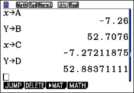
Begin by having the students graph a very simple curve such as y = x2 in the standard window of their calculator. Then TRACE to a point. Students will go to different points, some to the left and some to the right of the origin. ZOOM IN several times on this point until their graph appears linear (discuss local linearity here). To be sure they are on the graph push TRACE again. The coordinates of their point will be at the bottom of the screen; call this point (a, b). Return to the home screen and store the values to A and B (click here for instructions on storing and recalling numbers).

Return to the graph and push TRACE again to be sure the cursor is on the graph. Move the TRACE cursor one or two pixels away from the first point in either direction. This new point is (c, d). Return to the home screen and store the coordinates to C and D.

calc 2.1

Enter the equation of the line through the two points on the equation entry screen in terms of A, B, C, and D. Zoom Out several times until you have returned to the original window..

calc 2.4

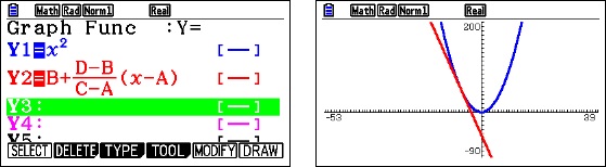
Exploration 1: Have students compare and contrast their graphs with several other students and discuss their observations. (Expected observations: the lines appear tangent at each students’ original point)

Exploration 2: Ask student to compute the slope of the line through their points, again using A, B, C, and D. Collect each student’s x-coordinate, A, and their slope and enter them in list is your calculator so that they can be projected.

calc 2.2

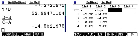
Study the two lists and discuss the relation is any. (Expected observations: the slope is twice the x-coordinate.) Can you write an equation of these pairs? (Expected result: y = 2x)

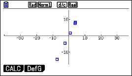
Finally, plot the points on the calculator using a square window. Do the points seem to lie on the line y =2x?

calc 2.3

Extensions:

Try the same activity with other functions such as y = (1/3)x3, y = x3, or y = x4. Anything more difficult will still result in a tangent line, but the numerical relationship between x and the slope will probably be too difficult to see. You may also consider y = sin(x) or y = cos(x). Again, the numerical work in Exploration 2, will be too difficult to see, but on graphing the points the result may be obvious. For y = sin(x), return to the list and add a column with the cosines of the x-values. Compare these with the slopes.

Advertisement

Concepts Related to Graphs

This and the next several posts will be about graphing and specifically how the function and its first and second derivatives are related. Since I do not intend this to be a textbook, I will not be doing textbook stuff. Rather, I hope to add some big picture things about the concepts involved. Hope you find it useful.

________________________________

Graphs of functions come in some combination of five shapes:

• Linear,
• Increasing, concave up,
• Increasing, concave down,
• Decreasing, concave up, and
• Decreasing, concave down.

I have put together an activity, An Exploration of the Shape of a Graph, to help students learn the relationship between the shapes and the derivative. Leaving the linear sections aside, the idea of the activity is to call students’ attention to the other four shapes and the slope of the tangent line (the derivative) in the intervals where the graph has each shape.

The key is to keep focused on the tangent line. To this end I suggest drawing short tangent segments parallel to the graph, as illustrated in the figure below.

Air-graphing: Another way to help students internalize this idea is to draw the graph of a function on the board and then have the students hold their pen out in front of them so the pen looks like a segment tangent to the graph. Then move the pen along the graph paying attention to the slope.

Either way what you want students to be aware of is

(1) Where the slopes are positive and where they are negative. This will later be related to the intervals where the function increases and decreases, and

(2) How the slope itself is changing. Is the slope increasing or decreasing? This will later be related to the concavity.

I hope you and your students find this activity helpful.

Local Linearity II

Using Local Linearity to introduce difference quotient and the derivative.

An effective way to introduce difference quotients and derivatives is to write the equation of the “line” you see when you zoom-in on a locally linear function.

First: Ask your class to use their calculator or computer grapher to graph a function, say y = sin(x), or some function they like better.

  1. Ask them to trace over to some point where the graph is “curvy.” (So they will remain on the graph, use the TRACE feature, not the moving cursor.) They do not have to go to, or even be near, the same place.
  2. Then ask them to zoom-in several times until their graph looks like a straight line (locally linear) and save the coordinates of that point as a and b (see the technology hint below).
  3. Then return to the graph and trace one or two clicks left or right to a nearby point on the graph and record the coordinates of that point as c and d.
  4. Write the equation of the line through (a, b) and (c ,d) and enter it in the graphing menu (see technology hint again).
  5. Graph the line. They should see only one “line” because the two graphs are on top of each other.
  6. Re-graph in the standard or Trig window. What do you see now? They should see their original graph with a line that appears tangent to it at the point (a, b).

Next: Discuss what you’ve done, specifically in finding the slope. The value c is a plus a little bit, that is c = a + h. (Or minus a  little bit if h is negative.) So the slope is

\displaystyle \frac{Y1(a+h)-Y1(a)}{(a+h)-a}\text{ or }\frac{f\left( x+h \right)-f\left( x \right)}{h}

and now you are ready to talk about difference quotients and their limit the derivative.

Technology Hints:

When you trace a graph on a calculator the coordinates of the point are written on the bottom of the screen as X and Y, or xc and yc. If you return to the home screen and type X [STO] A and Y [STO] B (or xc [STO] a etc.) the values will be saved to A and B. When you trace to the next point the x and y change, so return to the home screen and save them as C and D.

The line can be written directly in the equation editor in point-slope form by typing Y2 = Y1(A) + (Y1(B)-Y1(A))/(B – A)*(x – A)