Graph Analysis Questions (Type 3)

AP  Questions Type 3: Graph Analysis

The long name is “Here’s the graph of the derivative, tell me things about the function.”

Students are given either the equation of the derivative of a function or a graph identified as the derivative of a function with no equation is given. It is not expected that students will write the equation of the function from the graph (although this may be possible); rather, students are expected to determine key features of the function directly from the graph of the derivative. They may be asked for the location of extreme values, intervals where the function is increasing or decreasing, concavity, etc. They may be asked for function values at points. They will be asked to justify their conclusions.

The graph may be given in context and students will be asked about that context. The graph may be identified as the velocity of a moving object and questions will be asked about the motion. See Linear Motion Problems (Type 2)

Less often the function’s graph may be given, and students will be asked about its derivatives.

What students should be able to do:

  • Read information about the function from the graph of the derivative. This may be approached by derivative techniques or by antiderivative techniques.
  • Find and justify where the function is increasing or decreasing.
  • Find and justify extreme values (1st and 2nd derivative tests, Closed interval test a/k/a Candidates’ test).
  • Find and justify points of inflection.
  • Find slopes (second derivatives, acceleration) from the graph.
  • Write an equation of a tangent line.
  • Evaluate Riemann sums from geometry of the graph only. This usually involves familiar shapes such as triangles or semicircles.
  • FTC: Evaluate integral from the area of regions on the graph.
  • FTC: The function, g(x), may be defined by an integral where the given graph is the graph of the integrand, f(t), so students should know that if,

\displaystyle g\left( x \right)=g\left( a \right)+\int_{a}^{x}{{f\left( t \right)dt}}, then  \displaystyle {g}'\left( x \right)=f\left( x \right)  and  \displaystyle {g}''\left( x \right)={f}'\left( x \right).

In this case, students should write \displaystyle {g}'\left( x \right)=f\left( x \right) on their answer paper, so it is clear to the reader that they understand this.

Not only must students be able to identify these things, but they are usually asked to justify their answer and reasoning. See Writing on the AP Exams for more on justifying and explaining answers.

There are numerous ideas and concepts that can be tested with this type of question. The type appears on the multiple-choice exams as well as the free-response. Between multiple-choice and free-response this topic may account for 15% or more of the points available on recent tests. It is very important that students are familiar with all the ins and outs of this situation.

As with other questions, the topics tested come from the entire year’s work, not just a single unit. In my opinion many textbooks do not do a good job with integrating these topics, so be sure to use as many actual AP Exam questions as possible. Study past exams: look them over and see the different things that can be asked.

The Graph Analysis problem may cover topics primarily from primarily from Unit 4, Unit 5, and Unit 8 of the CED 

For previous posts on this subject see October 1517192426 (my most read post), 2012 and January 2528, 2013

Free-response questions:

  • Function given as a graph, questions about its integral (so by FTC the graph is the derivative):  2016 AB 3/BC 3, 2018 AB3
  • Table and graph of function given, questions about related functions: 2017 AB 6,
  • Derivative given as a graph: 2016 AB 3 and 2017 AB 3
  • Information given in a table 2014 AB 5
  • 2021 AB 4 / BC 4
  • 2021 AB 5 (b), (c), (d)
  • 2022 AB3 / BC3 – graph analysis, max/min
  • 2023 AB 4 / BC 4 – graph stem, max/min, concavity, L’Hospital’s Rule

Multiple-choice questions from non-secure exam. Notice the number of questions all from the same year; this is in addition to one free-response question (~25 points on AB and ~23 points on BC out of 108 points total)

  • 2012 AB: 2, 5, 15, 17, 21, 22, 24, 26, 76, 78, 80, 82, 83, 84, 85, 87
  • 2012 BC 3, 11, 12, 15, 12, 18, 21, 76, 78, 80, 81, 84, 88, 89

A good activity on this topic is here. The first pages are the teacher’s copy and solution. Then there are copies for Groups A, B, and C. Divide your class into 3 or 6 or 9 groups and give one copy to each. After they complete their activity have the students compare their results with the other groups.


Revised March 12, 2021, March 18, 2022, June 4, 2023


Advertisement

Reading the Derivative’s Graph

A very typical calculus problem is given the equation of a function, to find information about it (extreme values, concavity, increasing, decreasing, etc., etc.). This is usually done by computing and analyzing the first derivative and the second derivative. All the textbooks show how to do this with copious examples and exercises. I have nothing to add to that. One of the “tools” of this approach is to draw a number line and mark the information about the function and the derivative on it.

A very typical AP Calculus exam problem is given the graph of the derivative of a function, but not the equation of either the derivative or the function, to find all the same information about the function. For some reason, students find this difficult even though the two-dimensional graph of the derivative gives all the same information as the number line graph and, in fact, a lot more.

Looking at the graph of the derivative in the x,y-plane it is easy to determine the important information. Here is a summary relating the features of the graph of the derivative with the graph of the function.

Feature the function
{y}'> 0 is increasing
{y}' < 0 is decreasing
{y}' changes – to + has a local minimum
{y}'changes + to – has a local maximum
{y}' increasing is concave up
{y}' decreasing is concave down
{y}' extreme value has a point of inflection

Here’s a typical graph of a derivative with the first derivative features marked.

Here is the same graph with the second derivative features marked.

The AP Calculus Exams also ask students to “Justify Your Answer.” The table above, with the columns switched does that. The justifications must be related to the given derivative, so a typical justification might read, “The function has a relative maximum at x-2 because its derivative changes from positive to negative at x = -2.”

Conclusion Justification
y is increasing {y}'> 0
y is decreasing {y}'< 0
y has a local minimum {y}'changes  – to +
y has a local maximum {y}'changes + to –
y is concave up {y}'increasing
y is concave down {y}'decreasing
y has a point of inflection {y}'extreme values

For notes on asymptotes see Asymptotes and the Derivative and Other Asymptotes.

Originally posted on October 26, 2012, and my single most viewed post over the years.

Unit 5 – Analytical Applications of Differentiation

Unit 5 covers the application of derivatives to the analysis of functions and graphs. Reasoning and justification of results are also important themes in this unit. (CED – 2019 p. 92 – 107). These topics account for about 15 – 18% of questions on the AB exam and 8 – 11% of the BC questions.

You may want to consider teaching Unit 4 after Unit 5. Notes on Unit 4 are here.

Reasoning and writing justification of results are mentioned and stressed in the introduction to the topic (p. 93) and for most of the individual topics. See Learning Objective FUN-A.4 “Justify conclusions about the behavior of a function based on the behavior of its derivatives,” and likewise in FUN-1.C for the Extreme value theorem, and FUN-4.E for implicitly defined functions. Be sure to include writing justifications as you go through this topic. Use past free-response questions as exercises and also as guide as to what constitutes a good justification. Links in the margins of the CED are also helpful and give hints on writing justifications and what is required to earn credit. See the presentation Writing on the AP Calculus Exams and its handout

Topics 5.1

Topic 5.1 Using the Mean Value Theorem While not specifically named in the CED, Rolle’s Theorem is a lemma for the Mean Value Theorem (MVT). The MVT states that for a function that is continuous on the closed interval and differentiable over the corresponding open interval, there is at least one place in the open interval where the average rate of change equals the instantaneous rate of change (derivative). This is a very important existence theorem that is used to prove other important ideas in calculus. Students often confuse the average rate of change, the mean value, and the average value of a function – See What’s a Mean Old Average Anyway?

Topics 5.2 – 5.9

Topic 5.2 Extreme Value Theorem, Global Verses Local Extrema, and Critical Points An existence theorem for continuous functions on closed intervals

Topic 5.3 Determining Intervals on Which a Function is Increasing or Decreasing Using the first derivative to determine where a function is increasing and decreasing.

Topic 5.4 Using the First Derivative Test to Determine Relative (Local) Extrema Using the first derivative to determine local extreme values of a function

Topic 5.5 Using the Candidates’ Test to Determine Absolute (Global) Extrema The Candidates’ test can be used to find all extreme values of a function on a closed interval

Topic 5.6 Determining Concavity of Functions on Their Domains FUN-4.A.4 defines (at least for AP Calculus) When a function is concave up and down based on the behavior of the first derivative. (Some textbooks may use different equivalent definitions.) Points of inflection are also included under this topic.

Topic 5.7 Using the Second Derivative Test to Determine Extrema Using the Second Derivative Test to determine if a critical point is a maximum or minimum point. If a continuous function has only one critical point on an interval then it is the absolute (global) maximum or minimum for the function on that interval.

Topic 5.8 Sketching Graphs of Functions and Their Derivatives First and second derivatives give graphical and numerical information about a function and can be used to locate important points on the graph of the function.

Topic 5.9 Connecting a Function, Its First Derivative, and Its Second Derivative First and second derivatives give graphical and numerical information about a function and can be used to locate important points on the graph of the function.

Topics 5.10 – 5.11

Optimization is an important application of derivatives. Optimization problems as presented in most textbooks, begin with writing the model or equation that describes the situation to be optimized. This proves difficult for students, and is not “calculus” per se. Therefore, writing the equation has not been asked on AP exams in recent years (since 1983). Questions give the expression to be optimized and students do the “calculus” to find the maximum or minimum values. To save time, my suggestion is to not spend too much time writing the equations; rather concentrate on finding the extreme values.

Topic 5.10 Introduction to Optimization Problems 

Topic 5.11 Solving Optimization Problems

Topics 5.12

Topic 5.12 Exploring Behaviors of Implicit Relations Critical points of implicitly defined relations can be found using the technique of implicit differentiation. This is an AB and BC topic. For BC students the techniques are applied later to parametric and vector functions.


Timing

Topic 5.1 is important and may take more than one day. Topics 5.2 – 5.9 flow together and for graphing they are used together; after presenting topics 5.2 – 5.7 spend the time in topics 5.8 and 5.9 spiraling and connecting the previous topics. Topics 5.10 and 5.11 – see note above and spend minimum time here. Topic 5.12 may take 2 days.

The suggested time for Unit 5 is 15 – 16 classes for AB and 10 – 11 for BC of 40 – 50-minute class periods, this includes time for testing etc.

Finally, were I still teaching, I would teach this unit before Unit 4. The linear motion topic (in Unit 4) are a special case of the graphing ideas in Unit 5, so it seems reasonable to teach this unit first. See Motion Problems: Same thing, Different Context

This is a re-post and update of the third in a series of posts from last year. It contains links to posts on this blog about the differentiation of composite, implicit, and inverse functions for your reference in planning. Other updated post on the 2019 CED will come throughout the year, hopefully, a few weeks before you get to the topic. 


Previous posts on these topics include:

Then There Is This – Existence Theorems

What’s a Mean Old Average Anyway

Did He, or Didn’t He?   History: how to find extreme values without calculus

Mean Value Theorem

Foreshadowing the MVT

Fermat’s Penultimate Theorem

Rolle’s theorem

The Mean Value Theorem I

The Mean Value Theorem II

Graphing

Concepts Related to Graphs

The Shapes of a Graph

Joining the Pieces of a Graph

Extreme Values

Extremes without Calculus

Concavity

Reading the Derivative’s Graph

        Other Asymptotes

Real “Real-life” Graph Reading

Far Out! An exploration

Open or closed Should intervals of increasing, decreasing, or concavity be open or closed?

Others

Lin McMullin’s Theorem and More Gold  The Golden Ratio in polynomials

Soda Cans Optimization video

Optimization – Reflections   

Curves with Extrema?

Good Question 10 – The Cone Problem

Implicit Differentiation of Parametric Equations    BC Topic


Here are links to the full list of posts discussing the ten units in the 2019 Course and Exam Description.

Limits and Continuity – Unit 1  (8-11-2020)

Definition of t he Derivative – Unit 2  (8-25-2020)

Differentiation: Composite, Implicit, and Inverse Function – Unit 3  (9-8-2020)

Contextual Applications of the Derivative – Unit 4   (9-22-2002)   Consider teaching Unit 5 before Unit 4

Analytical Applications of Differentiation – Unit 5  (9-29-2020) Consider teaching Unit 5 before Unit 4 THIS POST

LAST YEAR’S POSTS – These will be updated in coming weeks

2019 – CED Unit 6 Integration and Accumulation of Change

2019 – CED Unit 7 Differential Equations  Consider teaching after Unit 8

2019 – CED Unit 8 Applications of Integration   Consider teaching after Unit 6, before Unit 7

2019 – CED Unit 9 Parametric Equations, Polar Coordinates, and Vector-Values Functions 

2019 CED Unit 10 Infinite Sequences and Series


Adapting 2021 AB 4 / BC 4

Four of nine. Continuing the series started in the last three posts, this post looks at the AP Calculus 2021 exam question AB 4 / BC 4. The series considers each question with the aim of showing ways to use the question with your class as is, or by adapting and expanding it.  Like most of the AP Exam questions there is a lot more you can ask from the stem and a lot of other calculus you can discuss.

2021 AB 4 / BC 4

This is a Graph Analysis Problem (type 3) and contains topics from Units 2, 4, and 6 of the current Course and Exam Description. The things that are asked in these questions should be easy for the students, however each year the scores are low. This may be because some textbooks simply do not give students problems like this. Therefore, supplementing with graph analysis questions from past exams is necessary.

There are many additional questions that can be asked based on this stem and the stems of similar problems. Usually, the graph of the derivative is given, and students are asked questions about the graph of the function. See Reading the Derivative’s Graph.

Some years this question is given a context, such as the graph is the velocity of a moving particle. Occasionally there is no graph and an expression for the derivative or function is given.

Here is the 2021 AB 4 / BC 4 stem:

The first thing students should do when they see G\left( x \right)=\int_{0}^{x}{{f\left( t \right)}}dt is to write prominently on their answer page {G}'\left( x \right)=f\left( x \right) and \displaystyle {G}''\left( x \right)={f}'\left( t \right). While they may understand and use this, they must say it.

Part (a): Students were asked for the open intervals where the graph is concave up and to give a reason for their answer. (Asking for an open interval is to remove any concern about the endpoints being included or excluded, a place where textbooks differ. See Going Up.)

Discussion and ideas for adapting this question:

  • Using this or similar graphs go through each of these with your class until the answers and reasons become automatic. There are quite a few other things that may be asked here based on the derivative.
    • Where is the function increasing?
    • Decreasing?
    • Concave down, concave up?
    • Where are the local extreme values?
    • What are the local extreme values?
    • Where are the absolute extreme values?
    • What are the absolute extreme values?
  • There are also integration questions that may be asked, such as finding the value of the functions at various points, such as G(1) = 2 found by using the areas of the regions. Also, questions about the local extreme values and the absolute extreme value including their values. These questions are answered by finding the areas of the regions enclosed by the derivative’s graph and the x-axis. Parts (b) and (c) do some of this.
  • Choose different graphs, including one that has the derivative’s extreme value on the x­-axis. Ask what happens there.

Part (b): A new function is defined as the product of G(x) and f(x) and its derivative is to be found at a certain value of x. To use the product rule students must calculate the value of G(x) by using the area between f(x) and the x-­axis and the value of {f}'\left( x \right) by reading the slope of f(x) from the graph.

Discussion and ideas for adapting this question:

  • This is really practice using the product rule. Adapt the problem by making up functions using the quotient rule, the chain rule etc. Any combination of \displaystyle G,{G}',{G}'',f,{f}',\text{ or }{f}'' may be used. Before assigning your own problem, check that all the values can be found from the given graph.
  • Different values of x may be used.

Part (c): Students are asked to find a limit. The approach is to use L’Hospital’s Rule.

Discussion and ideas for adapting this question:

  • To use L’Hospital’s Rule, students must first show clearly on their paper that the limit of the numerator and denominator are both zero or +/- infinity. Saying the limit is equal to 0/0 is considered bad mathematics and will not earn this point. Each limit should be shown separately on the paper, before applying L’Hospital’s Rule.
  • Variations include a limit where L’Hospital’s Rule does not apply. The limit is found by substituting the values from the graph.
  • Another variation is to use a different expression where L’Hospital’s Rule applies, but still needs values read from the graph.

Part (d): The question asked to find the average rate of change (slope between the endpoints) on an interval and then determine if the Mean Value Theorem guarantees a place where \displaystyle {G}' equals this value. Students also must justify their answer.

Discussion and ideas for adapting this question:

  • To justify their answer students must check that the hypotheses of the MVT are met and say so in their answer.
  • Adapt by using a different interval where the MVT applies.
  • Adapt by using an interval where the MVT does not apply and (1) the conclusion is still true, or (b) where the conclusion is false.

Next week 2021 AB 5.

I would be happy to hear your ideas for other ways to use this questions. Please use the reply box below to share your ideas.


Analytical Applications of Differentiation – Unit 5

Unit 5 covers the application of derivatives to the analysis of functions and graphs. Reasoning and justification of results are also important themes in this unit. (CED – 2019 p. 92 – 107). These topics account for about 15 – 18% of questions on the AB exam and 8 – 11% of the BC questions.

You may want to consider teaching Unit 4 after Unit 5. Notes on Unit 4 are here.

Reasoning and writing justification of results are mentioned and stressed in the introduction to the topic (p. 93) and for most of the individual topics. See Learning Objective FUN-A.4 “Justify conclusions about the behavior of a function based on the behavior of its derivatives,” and likewise in FUN-1.C for the Extreme value theorem, and FUN-4.E for implicitly defined functions. Be sure to include writing justifications as you go through this topic. Use past free-response questions as exercises and also as guide as to what constitutes a good justification. Links in the margins of the CED are also helpful and give hints on writing justifications and what is required to earn credit. See the presentation  Writing on the AP Calculus Exams and its handout

Topics 5.1

Topic 5.1 Using the Mean Value Theorem While not specifically named in the CED, Rolle’s Theorem is a lemma for the Mean Value Theorem (MVT). The MVT states that for a function that is continuous on the closed interval and differentiable over the corresponding open interval, there is at least one place in the open interval where the average rate of change equals the instantaneous rate of change (derivative). This is a very important existence theorem that is used to prove other important ideas in calculus. Students often confuse the average rate of change, the mean value, and the average value of a function – See What’s a Mean Old Average Anyway?

Topics 5.2 – 5.9

Topic 5.2 Extreme Value Theorem, Global Verses Local Extrema, and Critical Points An existence theorem for continuous functions on closed intervals

Topic 5.3 Determining Intervals on Which a Function is Increasing or Decreasing Using the first derivative to determine where a function is increasing and decreasing.

Topic 5.4 Using the First Derivative Test to Determine Relative (Local) Extrema Using the first derivative to determine local extreme values of a function

Topic 5.5 Using the Candidates’ Test to Determine Absolute (Global) Extrema The Candidates’ test can be used to find all extreme values of a function on a closed interval

Topic 5.6 Determining Concavity of Functions on Their Domains FUN-4.A.4 defines (at least for AP Calculus) When a function is concave up and down based on the behavior of the first derivative. (Some textbooks may use different equivalent definitions.) Points of inflection are also included under this topic.

Topic 5.7 Using the Second Derivative Test to Determine Extrema Using the Second Derivative Test to determine if a critical point is a maximum or minimum point. If a continuous function has only one critical point on an interval then it is the absolute (global) maximum or minimum for the function on that interval.

Topic 5.8 Sketching Graphs of Functions and Their Derivatives First and second derivatives give graphical and numerical information about a function and can be used to locate important points on the graph of the function.

Topic 5.9 Connecting a Function, Its First Derivative, and Its Second Derivative First and second derivatives give graphical and numerical information about a function and can be used to locate important points on the graph of the function.

Topics 5.10 – 5.11

Optimization is important application of derivatives. Optimization problems as presented in most text books, begin with writing the model or equation that describes the situation to be optimized. This proves difficult for students, and is not “calculus” per se. Therefore, writing the equation has not be asked on AP exams in recent years (since 1983). Questions give the expression to be optimized and students do the “calculus” to find the maximum or minimum values. To save time, my suggestion is to not spend too much time writing the equations; rather concentrate on finding the extreme values.

Topic 5.10 Introduction to Optimization Problems 

Topic 5.11 Solving Optimization Problems

Topics 5.12

Topic 5.12 Exploring Behaviors of Implicit Relations Critical points of implicitly defined relations can be found using the technique of implicit differentiation. This is an AB and BC topic. For BC students the techniques are applied later to parametric and vector functions.


Timing

Topic 5.1 is important and may take more than one day. Topics 5.2 – 5.9 flow together and for graphing they are used together; after presenting topics 5.2 – 5.7 spend the time in topics 5.8 and 5.9 spiraling and connecting the previous topics. Topics 5.10 and 5.11 – see note above and spend minimum time here. Topic 5.12 may take 2 days.

The suggested time for Unit 5 is 15 – 16 classes for AB and 10 – 11 for BC of 40 – 50-minute class periods, this includes time for testing etc.

Finally, were I still teaching, I would teach this unit before Unit 4. The linear motion topic (in Unit 4) are a special case of the graphing ideas in Unit 5, so it seems reasonable to teach this unit first. See Motion Problems: Same thing, Different Context

This is a re-post and update of the third in a series of posts from last year. It contains links to posts on this blog about the differentiation of composite, implicit, and inverse functions for your reference in planning. Other updated post on the 2019 CED will come throughout the year, hopefully, a few weeks before you get to the topic. 


Previous posts on these topics include:

Then There Is This – Existence Theorems

What’s a Mean Old Average Anyway

Did He, or Didn’t He?   History: how to find extreme values without calculus

Mean Value Theorem

Foreshadowing the MVT

Fermat’s Penultimate Theorem

Rolle’s theorem

The Mean Value Theorem I

The Mean Value Theorem II

Graphing

Concepts Related to Graphs

The Shapes of a Graph

Joining the Pieces of a Graph

Extreme Values

Extremes without Calculus

Concavity

Reading the Derivative’s Graph

        Other Asymptotes

Real “Real-life” Graph Reading

Far Out! An exploration

Open or Closed  Should intervals of increasing, decreasing, or concavity be open or closed?

Others

Lin McMullin’s Theorem and More Gold  The Golden Ratio in polynomials

Soda Cans  Optimization video

Optimization – Reflections   

Curves with Extrema?

Good Question 10 – The Cone Problem

Implicit Differentiation of Parametric Equations    BC Topic


Here are links to the full list of posts discussing the ten units in the 2019 Course and Exam Description.

Limits and Continuity – Unit 1  (8-11-2020)

Definition of t he Derivative – Unit 2  (8-25-2020)

Differentiation: Composite, Implicit, and Inverse Function – Unit 3  (9-8-2020)

Contextual Applications of the Derivative – Unit 4   (9-22-2002)   Consider teaching Unit 5 before Unit 4

Analytical Applications of Differentiation – Unit 5  (9-29-2020) Consider teaching Unit 5 before Unit 4 THIS POST

LAST YEAR’S POSTS – These will be updated in coming weeks

2019 – CED Unit 6 Integration and Accumulation of Change

2019 – CED Unit 7 Differential Equations  Consider teaching after Unit 8

2019 – CED Unit 8 Applications of Integration   Consider teaching after Unit 6, before Unit 7

2019 – CED Unit 9 Parametric Equations, Polar Coordinates, and Vector-Values Functions 

2019 CED Unit 10 Infinite Sequences and Series


Graph Analysis Questions (Type 3)

AP  Questions Type 3: Graph Analysis

The long name is “Here’s the graph of the derivative, tell me things about the function.”

Students are given either the equation of the derivative of a function or a graph identified as the derivative of a function with no equation is given. It is not expected that students will write the equation of the function from the graph (although this may be possible); rather, students are expected to determine important features of the function directly from the graph of the derivative. They may be asked for the location of extreme values, intervals where the function is increasing or decreasing, concavity, etc. They may be asked for function values at points. They will be asked to justify their conclusions.

The graph may be given in context and student will be asked about that context. The graph may be identified as the velocity of a moving object and questions will be asked about the motion. See Linear Motion Problems (Type 2)

Less often the function’s graph may be given and students will be asked about its derivatives.

What students should be able to do:

  • Read information about the function from the graph of the derivative. This may be approached by derivative techniques or by antiderivative techniques.
  • Find and justify where the function is increasing or decreasing.
  • Find and justify extreme values (1st and 2nd derivative tests, Closed interval test a/k/a Candidates’ test).
  • Find and justify points of inflection.
  • Find slopes (second derivatives, acceleration) from the graph.
  • Write an equation of a tangent line.
  • Evaluate Riemann sums from geometry of the graph only. This usually involves familiar shapes such as triangles or semicircles.
  • FTC: Evaluate integral from the area of regions on the graph.
  • FTC: The function, g(x), maybe defined by an integral where the given graph is the graph of  the integrand, f(t), so students should know that if,

\displaystyle g\left( x \right)=g\left( a \right)+\int_{a}^{t}{f\left( t \right)dt} then  {g}'\left( x \right)=f\left( x \right)  and  {{g}'}'\left( x \right)={f}'\left( x \right).

In this case, students should write {g}'(t)=f\left( t \right) on their answer paper, so it is clear to the reader that they understand this.

Not only must students be able to identify these things, but they are usually asked to justify their answer and reasoning. See Writing on the AP Exams for more on justifying and explaining answers.

The ideas and concepts that can be tested with this type question are numerous. The type appears on the multiple-choice exams as well as the free-response. Between multiple-choice and free-response this topic may account for 15% or more of the points available on recent tests. It is very important that students are familiar with all the ins and outs of this situation.

As with other questions, the topics tested come from the entire year’s work, not just a single unit. In my opinion many textbooks do not do a good job with integrating these topics, so be sure to use as many actual AP Exam questions as possible. Study past exams; look them over and see the different things that can be asked. The Graph Analysis problem may cover topics primarily from primarily from Unit 4, Unit 5, and Unit 8 of the 2019 CED 

For some previous posts on this subject see October 1517192426 (my most read post), 2012 and  January 2528, 2013

Free-response questions:

  • Function given as a graph, questions about its integral (so by FTC the graph is the derivative):  2016 AB 3/BC 3, 2018 AB3
  • Table and graph of function given, questions about related functions: 2017 AB 6,
  • Derivative given as a graph: 2016 AB 3 and 2017 AB 3
  • Information given in a table 2014 AB 5

Multiple-choice questions from non-secure exam. Notice the number of questions all from the same year; this is in addition to one free-response question (~25 points on AB and ~23 points on BC out of 108 points total)

  • 2012 AB: 2, 5, 15, 17, 21, 22, 24, 26, 76, 78, 80, 83, 82, 84, 85, 87
  • 2012 BC 3, 11, 12, 15, 12, 18, 21, 76, 78, 80, 81, 84, 88, 89

A good activity on this topic is here. The first pages are the teacher’s copy and solution. Then there are copies for Groups A, B, and C. Divide your class into 3 or 6 or 9 groups and give one copy to each. After they complete their activity have the students compare their results with the other groups.


Revised March 12, 2021


Good Question 17

A common question in (older?) textbooks is to give students a function or relation and have them graph it without technology (because in the old days technology was not available). Students had to find all the appropriate information without hints or further direction: they were supposed to know what to do and do it.

AP exam questions, for legitimate and understandable reasons, do not ask for as complete an analysis. Rather, they ask students to find specific information about the function or its graph (extreme values, points of inflection, etc.). For the same legitimate and understandable reason many of the features are not considered; the other concepts are tested on different questions.

I think that the full-analysis-from-scratch approach, while not appropriate for an AP exam question, has its merits. The big difference is that students need to be creative in their investigation; not just focus on a few items pointed to by the question.

With that in mind, let’s consider the following question asked three ways.

A very general form

Consider the relation {{x}^{3}}+3{{x}^{2}}+{{y}^{2}}=4. Discuss the graph of the relation giving reasons for your conclusions. Include a brief mention of any unproductive paths you followed and what you learned from them.
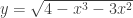
A more directed investigation

Consider the relation {{x}^{3}}+3{{x}^{2}}+{{y}^{2}}=4. Find its extreme values and any asymptotes, and vertical tangents (if any). Discuss in detail the appearance of the graph near x = –2 and discuss the slopes in that area. Explain how you arrived at your results.

Closer to an AP style form. The function here is the top half of the function above.

Consider the function y=\sqrt{{4-{{x}^{3}}-3{{x}^{2}}}}.

(a) Find the local maximum and minimum values of the function. Justify your answer.

(b) Where does the function had a vertical asymptote? Justify your answer.

(c) Find \underset{{x\to -2-}}{\mathop{{\lim }}}\,\frac{{dy}}{{dx}} and \underset{{x\to -2+}}{\mathop{{\lim }}}\,\frac{{dy}}{{dx}}. What does this say about the graph?

The real question is can you ask it the first way?

Here is my solution to the first form; this will also give the answers to the other forms. After the solution, I’ll discuss some ideas on how to score such a solution.

Solution

The graph of the relation  {{x}^{3}}+3{{x}^{2}}+{{y}^{2}}=4.  is shown in figure 1.

Figure 1

The domain of the function is x\le 1
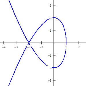
. Values greater than 1 will make the left side of the equation greater than 4 regardless of the value of y. The range of the relation is all real numbers.

The function is symmetric to the x-axis since substituting (–y) for y will give the same expression. The equation of the top half is  y=\sqrt{{4-{{x}^{3}}-3{{x}^{2}}}} and the lower half is y=-\sqrt{{4-{{x}^{3}}-3{{x}^{2}}}}

The derivative for the top half is \displaystyle {y}'=-\frac{{3{{x}^{2}}+6x}}{{2y}}=-\frac{{3{{x}^{2}}+6x}}{{2\sqrt{{4-{{x}^{3}}-{3{x}^{2}}}}}} 
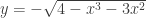
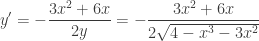
by implicit differentiation or by differentiating the equation for the top half.

y'\left( x \right) does not exist at x = 1 specifically, \displaystyle \underset{{x\to 1-}}{\mathop{{\lim }}}\,{y}'\left( x \right)=-\infty . Therefore, the line x = 1 is a vertical tangent. By symmetry for the lower part of the graph \displaystyle \underset{{x\to 1-}}{\mathop{{\lim }}}\,{y}'\left( x \right)=+\infty 
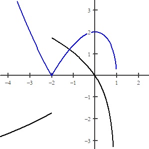
.  And x = 1 is its vertical asymptote as well. The slope of the original relation changes from positive to negative at x = 1 by going not through zero but from  -\infty to +\infty .

{y}'\left( x \right)=0 when x = 0 and when x = –2. At (0, 2) the derivative changes from positive to negative; this is a local maximum point by the first derivative test. The lower half has a local minimum point at (0, –2) by symmetry.

At (–2, 0) the derivative is an indeterminate form of the type 0/0.

False step: At first, I thought this meant that the two sides were tangent to the line x = –2 making the point (–2, 0) on the top half a cusp. I tried to see if this was true by graphing in a very narrow window. This did not show anything: the graph looked on zooming in, like an absolute value graph. It turned out that an absolute value was involved.

I then made a table of values for the derivative near the point and found that the values appeared to be approaching a number near –1.7 from the left and near +1.7 from the right. I started thinking maybe \displaystyle \sqrt{3}.

Then I changed the constants to parameters and played with the sliders on Desmos (here). With a slight change in the constants the graph appeared to have a nice rounded local minimum near x= –2. Other values showed two separate pieces with vertical tangents near x= –2. This confused me even more.

Next, I did what I should have done earlier: I graphed the top half and its derivative (figure 2):

Figure 2. The top half in blue and its derivative in black.

The derivative has a finite jump discontinuity at x = –2. I remembered seeing this kind of thing before and thought it involved an absolute value of some kind. Still confused, I decided to investigate the derivative further (which I also should have done sooner).

The derivative at x = –2 is an indeterminate form of the 0/0 type. This means that by substituting you get an expression that really doesn’t help; you may still evaluate the limit (remember derivatives are limits) by other methods. Factoring the derivative (using synthetic division on the radicand) gives

\displaystyle {y}'\left( x \right)=-\frac{{3x\left( {x+2} \right)}}{{2\sqrt{{{{{\left( {x+2} \right)}}^{2}}\left( {1-x} \right)}}}}=-\frac{{3x\left( {x+2} \right)}}{{2\sqrt{{{{{\left( {x+2} \right)}}^{2}}}}\sqrt{{1-x}}}}=-\frac{{3x}}{{\sqrt{{1-x}}}}\frac{{x+2}}{{\left| {x+2} \right|}}

And now we see that

\displaystyle \underset{{x\to -2-}}{\mathop{{\lim }}}\,\frac{{-3x}}{{2\sqrt{{1-x}}}}\cdot \frac{{x+2}}{{\left| {x+2} \right|}}=-\sqrt{3}  and  \displaystyle \underset{{x\to -2+}}{\mathop{{\lim }}}\,\frac{{-3x}}{{2\sqrt{{1-x}}}}\cdot \frac{{x+2}}{{\left| {x+2} \right|}}=\sqrt{3}

This agrees with the derivative’s graph. The top graph (and bottom’s by symmetry) comes to an arrow-like point (sometimes called a node) at (–2, 0). The slope on the left approaches -\sqrt{3} and on the right approaches +\sqrt{3}.

______________________

I admit I’ve had a few more years of experience with this sort of thing that a first-year calculus student. I expect this would be difficult for most students who have never seen a question like this, so working up to it with simpler questions is how to start.

In grading this sort of question, you need to consider:

  1. If the student found and justified all the pertinent features of the graph. If they missed something, what they included may still be pretty good. For example, I would not expect a student to the use the word “node,” so omitting it should not be held against them and using it may call for praise.
  2. The things they (and I) may have overlooked or things they considered that were unnecessary or even wrong.
  3. Their overall approach. This last may be the most important part. Including their missteps and unproductive paths is important and should, I think, receive credit. After all, they did not know the path would be unproductive until they followed it a way. Hopefully, they made some missteps and learned something from them. That’s what investigating something in math entails.

I would be happy to hear if you tried this or something similar and so would the other readers of this blog. Please use the “Comment” button below to share your thoughts.