The fifth in the Graphing Calculator / Technology series
(The MPAC discussion will continue next week)
Seeing discontinuities on a graphing calculator is possible; but you need to know how a calculator graphs to do it. Here’s the story:
The number you choose for XMIN becomes the x-coordinate of the (center of) the pixels in the left most column of pixels. The number you choose for XMAX is the x-coordinate of the right most column of pixels. The distance between XMIN and XMAX is divided evenly between the remaining pixels so that all the pixels are evenly spaced across the screen (the same distance apart). The rows of pixels are done the same way evenly spacing them between YMIN and YMAX.
This spacing is usually not at “nice” values as can be seen by just moving the cursor across the screen and noticing the x-values or y-values at the bottom of the screen.

The cursor is located one pixel to the right of the y-axis and one pixel above the x-axis in the “standard” window of a TI-8x. Note the coordinates of that pixel at the bottom of the screen. These are the distances between the pixels.
To draw a graph, the calculator takes the x-coordinate of each pixel, calculates the corresponding y-value and turns on the pixel in that column with closest y-pixel-coordinate. If set in a connect mode, the calculator turns on several pixels in adjacent columns so that the y-values seem to connect; this is why the graph often looks jagged in steep sections of the graph. If you are in DOT mode, this does not happen and only one pixel in each column is on.
If you move the cursor over one of the points on a graph, you will see the pixel coordinates, NOT the actual y-coordinates. Use TRACE to see the actual y-coordinate. This is why when finding intersections, you should not just move the cursor over the point, but rather use “intersect” to see the actual y-value of the function.
If the function is undefined for some x-pixel value, then no pixel will turn on in that column. If the function is undefined for some value between the pixel values, then nothing happens because the calculator has not evaluated the function there, so the graph seems to be continuous.
Vertical “asymptotes” are the result of the calculator not evaluating the function at the undefined value; rather it connects the value on one side of the asymptote off the bottom of the screen with the next value on the other side of the asymptote off the top of the screen. If the asymptote appears exactly at a pixel value, then no “asymptote” will appear and that column of pixels will have no pixel turned on. (Some newer calculators and newer operating systems on older calculators have made adjustments so that the “asymptotes” do not show up. In some systems this feature can be turned on or off.)

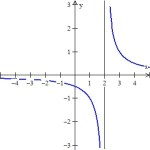
The function  in the standard window. The vertical line is not really the asymptote and the “hole” at (2, 0.75) is not seen.
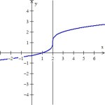
A removable discontinuity, a hole in the graph (really a skipped pixel), can be seen, if it occurs at a pixel value. Since in most examples the hole is at an integer or other “nice” number, you will not see them in the “standard” window. Use a “decimal” window, which has been chosen in advance so the x-values of the pixels are integers and nice decimals. (To see this, in a decimal window move the cursor around and notice the pixel coordinates).
The other thing you can do is adjust the XMIN and XMAX values so that the distance between them will land on integer values. (Nice project for your class – the number of pixels can be found in the guidebook, or you can count them. In the old days, before decimal windows, this was necessary – it was called finding a “friendly window.”)

The function in the “decimal” window. The “asymptote” has disappeared and the “hole” at (2, 0.75) is now visible.
Zooming in or out may change these values so the hole or asymptote disappears.
For a related idea see the post My Favorite Function
PLEASE NOTE: I have no control over the advertising that appears on this blog. It is provided by WordPress and I would have to pay a great deal to not have advertising. I do not endorse anything advertised here. I noticed that ads for one of the presidential candidates occasionally appears; I certainly do not endorse him.


![\displaystyle f\left( x \right)=\sqrt[3]{x}](https://s0.wp.com/latex.php?latex=%5Cdisplaystyle+f%5Cleft%28+x+%5Cright%29%3D%5Csqrt%5B3%5D%7Bx%7D&bg=ffffff&fg=333333&s=0&c=20201002)


 has an even vertical asymptote at x = 2. (Figure 1)
 has an odd vertical asymptote at x = 2. (Figure 2) Likewise, the tangent, cotangent, secant, and cosecant functions have odd vertical asymptotes.
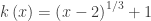
![\displaystyle h\left( x \right)=\sqrt[3]{{{{{\left( {x-2} \right)}}^{2}}}}+1](https://s0.wp.com/latex.php?latex=%5Cdisplaystyle+h%5Cleft%28+x+%5Cright%29%3D%5Csqrt%5B3%5D%7B%7B%7B%7B%7B%5Cleft%28+%7Bx-2%7D+%5Cright%29%7D%7D%5E%7B2%7D%7D%7D%7D%2B1&bg=ffffff&fg=333333&s=0&c=20201002)
 at (2,0) (Figure 4).
![\displaystyle z\left( x \right)=\left\{ {\begin{array}{*{20}{c}} {\sqrt[3]{{{{{\left( {x-2} \right)}}^{2}}}}-1} & {x<2} \\ {\sqrt[3]{{{{{\left( {x-2} \right)}}^{2}}}}+1} & {x\ge 2} \end{array}} \right.](https://s0.wp.com/latex.php?latex=%5Cdisplaystyle+z%5Cleft%28+x+%5Cright%29%3D%5Cleft%5C%7B+%7B%5Cbegin%7Barray%7D%7B%2A%7B20%7D%7Bc%7D%7D+%7B%5Csqrt%5B3%5D%7B%7B%7B%7B%7B%5Cleft%28+%7Bx-2%7D+%5Cright%29%7D%7D%5E%7B2%7D%7D%7D%7D-1%7D+%26+%7Bx%3C2%7D+%5C%5C+%7B%5Csqrt%5B3%5D%7B%7B%7B%7B%7B%5Cleft%28+%7Bx-2%7D+%5Cright%29%7D%7D%5E%7B2%7D%7D%7D%7D%2B1%7D+%26+%7Bx%5Cge+2%7D+%5Cend%7Barray%7D%7D+%5Cright.&bg=ffffff&fg=333333&s=0&c=20201002)
 and
and 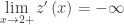 . Compare this with h(x) above.


 near x = 3 and as
  . Relate the values and their signs to the graph. (Divide by a small number get a big number; divide by a big number, get a small number.)
 has no value at x = 2 (f(2) does not exist), but as you get closer to x = 2 the function value gets closer to 4 (
 ).
). with a gap or hole at the point (2, 4). Another example:
 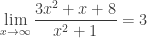 since, the graph gets closer to y = 3 as you go farther to the right. The line y = 3 is a horizontal asymptote.
 and since the fraction gets smaller as |x| gets larger, the function approaches 3 from above when x > 0 and from below when x < 0 (why?)
