Other Asymptotes

A few days ago, a reader asked if you could find the location of horizontal asymptotes from the derivative of a function. The answer, alas, is no. You can determine that a function has a horizontal asymptote from its derivative, but not where it is. This is because a function and its many possible vertical translations have the same derivative but different horizontal asymptotes. To locate it precisely, we need more information, an initial condition (a point on the curve).

I have written a post about the relationship between vertical asymptotes and the derivative of the function here. Today’s post will discuss horizontal asymptotes and their derivatives.

Definition: a straight line associated with a curve such that as a point moves along an infinite branch of the curve the distance from the point to the line approaches zero and the slope of the curve at the point approaches the slope of the line. (Merriam-Webster dictionary). Thus, asymptotes can be vertical, horizontal, or slanted.

Horizontal Asymptotes

Horizontal asymptotes are a form of end behavior: they appear as \displaystyle x\to \infty or \displaystyle x\to -\infty . Specifically, if a function has a horizontal asymptote(s), then \displaystyle \underset{{x\to \pm \infty }}{\mathop{{\lim }}}\,{f}'\left( x \right)=0,  At an asymptote, the curve must approach a horizontal line, therefore its slope must be approaching zero as \displaystyle x\to \infty or \displaystyle x\to -\infty .  The converse is not true: If the derivative approaches zero, the function may not have a horizontal asymptote. A counterexample is \displaystyle f\left( x \right)=\sqrt[3]{x}.

In the first four examples that follow, the derivative approaches 0 as \displaystyle x\to \infty and/or \displaystyle x\to -\infty

Example 1: \displaystyle {f}'\left( x \right)=\frac{1}{{1+{{x}^{2}}}}  (Figure 1 in blue).This is the derivative of \displaystyle f\left( x \right)={{\tan }^{{-1}}}(x),\ -\tfrac{\pi }{2}<f\left( x \right)<\tfrac{\pi }{2}. (Figure 1 in red). We see that the derivative approaches zero in both directions, this tells us that there may be horizontal asymptote(s). We must look at the function to find where they are: \displaystyle y=\tfrac{\pi }{2} and \displaystyle y=-\tfrac{\pi }{2}

Advertisement

Continuity

Karl Weierstrass (1815 – 1897) was the mathematician who (finally) formalized the definition of continuity. In that definition was the definition of limit. So, which came first – continuity or limit? The ideas and situations that required continuity could only be formalized with the concept of limit. So, looking at functions that are and are not continuous helps us understand what limits are and why we need them.

In the ideal world I mentioned last week, students would have plenty of work with continuous and not continuous functions. The vocabulary and notation, if not the formal definitions, would be used as early as possible. Then when students got to calculus, they would know the ideas and be ready to formalize the.

Using the definition of continuity to show that a function is or is not continuous at a point is a common question of the AP exams.

Continuity The definition of continuity.

Continuity Should continuity come before limits?

From One Side or the Other One-sided limits and one-sided differentiability

How to Tell Your Asymptote from a Hole in the Graph  From the technology series. Showing holes and asymptotes on a graphing calculator.

Fun with Continuity Defined everywhere and continuous nowhere. Continuous only at a single point.

Intermediate Weather  Using the IVT

Right Answer – Wrong Question Continuity or continuity on its domain


A Family of Functions

Good Question 2, continued. 

Today we continue looking at Good Question 2 from our last post. The jumping off place was the BC calculus exam question 5 from 2002. We looked at the differential equation \displaystyle \frac{dy}{dx}=2y-4x and its slope field and discussed the questions asked on the exam. Then we saw how to actually solve the equation and found the general solution to be y\left( x \right)=C{{e}^{2x}}+2x+1.

The general solution of a differential equation contains a constant and therefore defines a family of functions all of whom satisfy the differential equation; they have similar, but slightly different graphs. Let’s look at and discuss the similarities and differences.

In using this with a class I suggest you present it step by step with lots of questions (more than I have here) to help them find the way to the full description of the family of functions. Alternatively, you could be very general and ask them to discuss (and justify) end behavior and the location of any extreme values or other interesting features individually or in small groups.

The Rule of Four says that all mathematical situations should be looked at analytically (i.e. with equations), graphically, numerically and verbally. In the previous post the analytic considerations were foremost and the slope field accounted for the graphical aspect. Euler’s method was numerical. Today the numerical comes to the forefront to help us discuss the graph. (Fro the verbal, well, I’ve never been accused of not being verbose, writing-wise.)

The two numbers that need to be considered are the parameter C and numerical size of e2x.

When C = 0 the solution reduces to y = 2x + 1. This is a line. If we rewrite the general solution as y\left( x \right)=\left( 2x+1 \right)+C{{e}^{2x}} and realize that e2x is always positive, we can see that solutions with C > 0 lie above the line and those with C < 0 lie below.

Left end behavior

Look at the x-values moving from the origin to the left; where x is negative and getting larger in absolute value. Here e2x will get very small and the solution will all get closer to the line y = 2x + 1. If C > 0 the solutions will be a little above the line and if C < 0 they will lie just below the line.

Therefore, the left end behavior is that the functions approach y = 2x + 1 as a slant asymptote.

Maximum Points

In the previous post we determined that the origin was a maximum point of the solution that contained the origin (C = –1).  Are there extreme points for any other solutions?

The maximums occur where \displaystyle \frac{dy}{dx}=0, that is where 2y-4x=0 or y=2x. We know they are maximums by the second derivative test: \displaystyle \frac{{{d}^{2}}y}{d{{x}^{2}}}=2\frac{dy}{dx}-4=4C{{e}^{2x}}-2<0 when C  < 0. All the curves with C < 0 are concave down on their entire domain.

What does this mean? It means that for all the members of the family of solutions that have C < 0 have a maximum point, and that maximum point will be on the line y=2x.

Which members of the family can have maximums? Since y=2x lies below y=2x+1 only those with C < 0 will have maximums.

"Thirty

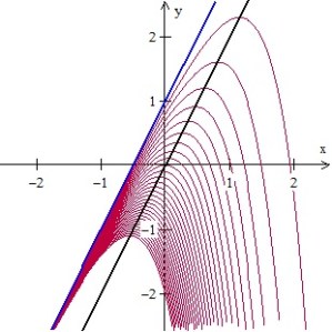
The graph above shows 30 members of the family with C = –3 (bottom curve) to C = –0.1 (top curve). The equation of the black line is y= 2x and the equation of the blue line is y= 2x + 1. Note that all the maximum points lie on the line y= 2x.

The curves with C > 0 lie above the line y= 2x + 1. For these curves \displaystyle \frac{{{d}^{2}}y}{d{{x}^{2}}}=2\frac{dy}{dx}-4=2\left( 2y-4x \right)-4=4y-8x-4

This expression will be positive when 4y-8x-4>0 or y>2x+1. In other words, when the curve lies above the line y= 2x + 1, exactly those with C > 0.

Therefore, all of these members of the family are concave up everywhere and since there is nowhere where their derivative is zero, there are no minimum points. See the graph below
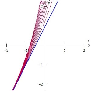
Ten family members from C=0.3 (bottom curve) to C = 30 (top)

Ten family members
from C = 0.3 (bottom curve) to C = 30 (top)

Right end behavior

From what we have determined above for C > 0 \displaystyle \underset{x\to \infty }{\mathop{\lim }}\,y\left( x \right)=\infty , and for C < 0, \displaystyle \underset{x\to \infty }{\mathop{\lim }}\,y\left( x \right)=-\infty .


When graphing calculators were first required on the AP calculus exams (1995) there were, for a few years, questions asking students to analyze some aspect of a family of functions. See for example 1995 BC 5, 1996 AB4/BC4, 1997 AB 4, 1997 BC 4, 1998 AB2/BC2. They seem to have stopped asking such questions. Too bad; there is some interesting calculus to be had in family of function questions.

Asymptotes

Horizontal asymptotes are the graphical manifestation of limits as x approaches infinity. Vertical asymptotes are the graphical manifestation of limits equal to infinity (at a finite x-value).

Thus, since \displaystyle \underset{x\to \infty }{\mathop{\lim }}\,\left( 1-{{2}^{-x}} \right)=1. The graph will show a horizontal asymptote at y = 1.

Since the graph of \displaystyle y={{2}^{-x}}\sin \left( x \right) approaches the x-axis as an asymptote, it follows that \underset{x\to \infty }{\mathop{\lim }}\,\left( {{2}^{-x}}\sin \left( x \right) \right)=0. (The fact that this graph crosses the x-axis many times on its trip to infinity is not a concern; the axis is still an asymptote.)

Since \underset{x\to 0}{\mathop{\lim }}\,\frac{1}{{{x}^{2}}}=\infty ,\underset{x\to {{0}^{-}}}{\mathop{\lim }}\,\frac{1}{x}=-\infty ,\text{ and }\underset{x\to {{0}^{+}}}{\mathop{\lim }}\,\frac{1}{x}=\infty , the functions all have a vertical asymptote of x = 0.


Why Limits?

There are four important things before calculus and in beginning calculus for which we need the concept of limit.

    1. The first is continuity. Most of the time in pre-calculus mathematics and in the calculus we deal with nice continuous functions or functions that are not continuous at just a few points. Limits give us the vocabulary and the mathematics necessary to describe and deal with discontinuities of functions. Historically, the modern (delta-epsilon) definition of limit comes out of Weierstrass’ definition of continuity.
    2. Asymptotes: A vertical asymptote is the graphical feature of function at a point where its limit equals positive or negative infinity. A horizontal asymptote is the (finite) limit of a function as x approaches positive or negative infinity.

Ideally, one would hope that students have seen these phenomena and have used the terms limit and continuity informally before they study calculus. This is where the study of calculus starts. The next two items are studied in calculus and are based heavily on limit.

3. The tangent line problem. The definition of the derivative as the limit of the slope of a secant line to a graph is the first of the two basic ideas of the calculus. This single idea is the basis for all the concepts and applications of differential calculus.

4. The area problem. Using limits it is possible to find the area of a region with a curved side, even if the curve is not something simple like a semi-circle. The definite integral is defined as the limit of a Riemann sum and gives the area regions with a curved side. This then can be extended to huge number of very practical applications many having nothing to do with area.

So these are the main ways that limits are used in beginning calculus. Students need a good visual  understanding, what the graph looks like,  of the first two situations listed above and how limits describe and define them. This is also necessary later when third and fourth come up.