Adapting 2021 AB 3 / BC 3

Three of nine. Continuing the series started in the last two posts, this post looks at the AB Calculus 2021 exam question AB 3 / BC 3. The series considers each question with the aim of showing ways to use the question in with your class as is, or by adapting and expanding it. Like most of the AP Exam questions there is a lot more you can ask from the stem and a lot of other calculus you can discuss.

2021 AB 3 / BC 3

This question is an Area and Volume question (Type 4) and includes topics from Unit 8 of the current Course and Exam Description. Typically, students are given a region bounded by a curve and an line and asked to find its area and its volume when revolved around a line. But there is an added concept here that we will look at first.

The stem is:

First, let’s consider the c. This is a family of functions question. Family of function questions appear now and then. They are discussed in the post on Other Problems (Type 7) and topics from Unit 8 of the current Course and Exam Description. My favorite example is 1998 AB 2, BC 2. Also see Good Question 2 and its continuation.

If we consider the function with c = 1 to be the parent function \displaystyle P\left( x \right)=x\sqrt{{4-{{x}^{2}}}} then the other members of the family are all of the form \displaystyle c\cdot P\left( x \right). The c has the same effect as the amplitude of a sine or cosine function:

  • The x-axis intercepts are unchanged.
  • If |c| > 1, the graph is stretched away from the x-axis.
  • If 0 < |c| < 1, the graph is compressed towards the x-axis.
  • And if c < 0, the graph is reflected over the x-axis.

All of this should be familiar to the students from their work in trigonometry. This is a good place to review those ideas. Some suggestions on how to expand on this will be given below.

Part (a): Students were asked to find the area of the region enclosed by the graph and the x-axis for a particular value of c. Substitute that value and you have a straightforward area problem.

Discussion and ideas for adapting this question:

  • The integration requires a simple u-substitution: good practice.
  • You can change the value of c > 0 and find the resulting area.
  • You can change the value of c < 0 and find the resulting area. This uses the upper-curve-minus-the-lower-curve idea with the upper curve being the x-axis (y = 0).
  • Ask students to find a general expression for the area in terms of c and the area of P(x).
  • Another thing you can do is ask the students to find the vertical line that cuts the region in half. (Sometimes asked on exam questions).
  • Also, you could ask for the equation of the horizontal line that cuts the region in half. This is the average value of the function on the interval. See these post 1, 2, 3, and this activity 4.

Part (b): This question gave the derivative of y(x) and the radius of the largest cross-sectional circular slice. Students were asked for the corresponding value of c. This is really an extreme value problem. Setting the derivative equal to zero and solving the equation gives the x-value for the location of the maximum. Substituting this value into y(x) and putting this equal to the given maximum value, and you can solve for the value of c.  

(Calculating the derivative is not being tested here. The derivative is given so that a student who does not calculate the derivative correctly, can earn the points for this part. An incorrect derivative could make the rest much more difficult.)

Discussion and ideas for adapting this question:

  • This is a good problem for helping students plan their work, before they do it.
  • Changing the maximum value is another adaption. This may require calculator work; the numbers in the question were chosen carefully so that the computation could be done by hand. Nevertheless, doing so makes for good calculator practice.

Part (c): Students were asked for the value of c that produces a volume of 2π. This may be done by setting up the volume by disks integral in terms of c, integrating, setting the result equal to 2π, and solving for c.

Discussion and ideas for adapting this question:

  • Another place to practice planning the work.
  • The integration requires integrating a polynomial function. Not difficult, but along with the u-substitution in part (a), you have an example to show people that students still must do algebra and find antiderivatives.
  • Ask students to find a general expression for the volume in terms of c and the volume of P(x).
  • Changing the given volume does not make the problem more difficult.

Next week 2021 AB 3/ BC 3.

I would be happy to hear your ideas for other ways to use this questions. Please use the reply box below to share your ideas.


Advertisement

Quadratic Formula or Not?

There was a very interesting post in the AP Calc TEACHERS – AB/BC Facebook page last week. It discussed an apparently new method for solving quadratic equation without guess-and-check factoring, completing the square, or the quadratic formula. It was discovered by Dr. Po-Shen Loh of Carnegie Mellon University. The full article is here. The article links to a video of Dr. Loh explaining his method.

This method will work for any and all quadratic equations and is easy, almost intuitive, to understand. Folks have been solving quadratics in the West since long before Euclid’s time, in Muslin countries, in India, and in China. It is a surprise no one found this method before.

I’ll show you the method (an algorithm really). It is based on long known fact that for a quadratic equation in the form

{{x}^{2}}+px+q=0

the sum of the roots is –p, the opposite of the coefficient of the first degree-term, and the constant term, q, is the product of the root.

Example 1 (A simple example to show the method): Solve  {{x}^{2}}+6x-16=0

  • The sum of the roots is –6.
  • Therefore, the average of the roots is –3
  • Since there are only 2 roots, they must be the same distance of either side of –3. Let the roots be \left( {-3+u} \right) and \left( {-3-u} \right) with \displaystyle u\ge 0.
  • The product of the roots is \left( {-3+u} \right)\left( {-3-u} \right)=-16
  • Solving this equation:

9-{{u}^{2}}=-16

{{u}^{2}}=25

u=5

  • Then the roots are –3 + 5 = 2 and –3 – 5 = –8

Example 2 (More complicated, but no more difficult) Solve 3{{x}^{2}}-7x+8=0

  • The leading coefficient must be 1, so divide by 3: {{x}^{2}}-\frac{7}{3}x+\frac{8}{3}=0
  • The average of the roots is 7/6.
  • The roots are \left( {\frac{7}{6}-u} \right) and \left( {\frac{7}{6}+u} \right)
  • Solving

\displaystyle \left( {\frac{7}{6}+u} \right)\left( {\frac{7}{6}-u} \right)=\frac{8}{3}

\displaystyle \frac{{49}}{{36}}-{{u}^{2}}=\frac{8}{3}

\displaystyle {{u}^{2}}=\frac{{49}}{{36}}-\frac{8}{3}=-\frac{{47}}{{36}}

\displaystyle u=\frac{{\sqrt{{47}}}}{6}i

  • And the roots are  \displaystyle \frac{7}{6}+\frac{{\sqrt{{47}}}}{6}i  and  \displaystyle \frac{7}{6}-\frac{{\sqrt{{47}}}}{6}i

You may even prove the quadratic formula using this method. I’ll leave that for something to do over vacation – Don’t worry, it won’t take long.

Happy Holidays to everyone.


BTW My next posts will  be in January about Units 9 and 10 of the AP Calculus Course Description.


Spiral Slide Rule

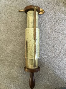
As I wrote last week, I found an old spiral slide rule last summer. It is about the size of a rolling pin and in fact has a handle like a rolling pin’s at the bottom. The device consists of a short wide cylinder that slides around, and up or down on a longer thin cylinder.

The short wide cylinder has a spiral common (base 10) logarithm scale starting at the top at the 100 mark after the words “slide rule” (see Figure 3). The scale runs around the cylinder 50 times ending precisely under the starting mark. By my measurement the scale is about 511 inches or 42.6 feet long. (1.30 meters). The scale is marked for 4 digits reading with a 5th digit that can be reasonably estimated. (By way of comparison, the common 10-inch slide rule scale discussed last week allows for 2 digits reading with the third digit estimated.) These are the mantissas of the common logarithms from 1 at the zero point (since log (1) = 0) to 1.0 (log (10) = 1) at the lower end.

The thin cylinder is marked with several formulas and other information including a table of natural sines from 0 to 45 degrees, from which you can have the value of any trig function if you’re clever enough. This cylinder is not used for calculations; it is there to allow the wider cylinder to move.

There are also two pointers. The shorter one is attached to the bottom and fixed. The cylinder is moved into position for this pointer. The longer pointer is attached to the thin cylinder and can be moved to the position needed – up, down left or right. Both the top end and the bottom end of the long pointer may be used. The pointers are made to slide past each other if necessary. If the long pointer covers the number needed the other side of it may be used instead (just don’t switch back-and-forth in the same computation).

Here is how it works. For the multiplication problem 15.115 x 439.65.

For the moment we ignore the decimal points.

  1. The top, “T” shaped, pointer is moved to the start value after “Slide rule.”
  2. The bottom pointer is first set at 15115 (the 151 is marked, the next 1 is the first mark following 151 and the 5 is estimated. See Figure 3 (Click to enlarge). The distance between the two measured almost 9 times around the cylinder is log (1.5115)
  3. Next the cylinder is moved without disturbing the pointers so that the top pointer is at 4.3965 and again estimating the last digit. Figure 4 upper long pointer.
  4. The product is at the fixed pointer: 6.645 Figure 4 lower pointer.
  5. Finally, we put the decimal in the proper place. The product is 6645.
  6. The full value is 6645.30975 by calculator. So the answer is correct to 4 digits, good enough for most practical work.

By moving the top pointer to log (4.3965) and using the pointers to add to it log (1.5115) we have performed the calculation log (1.5115) + log (4.3965) = log (1.5115. x 4.3965) = log (6.645)

To divide the procedure is reversed.  \frac{{6645}}{{439.65}}

  1. Set the fixed pointer to the dividend and move the top pointer to one of the divisors. (Figure 4)
  2. Without moving the pointers, move the cylinder so the top pointer is at 1.
  3. The quotient is at the fixed pointer (Figure 3)
  4. Adjust the decimal point for the quotient: 15.115.

If the cylinder is moved so that the pointer is off the bottom of the cylinder, the bottom pointer is used instead of the top. (This is the reason it is directly below the top pointer.)

If this seems like a lot of trouble, it is. But remember, a working computer was not available until near the end of World War II and filled a room. Electronic calculators were not available until around 1970. Computations before then were done by hand or with logarithms.

When I was in college in the early 1960s, I worked for an engineer on my summer vacations. My boss had and occasionally used a large table of logarithms. Large, as in a whole book! As I recall, it was good without interpolating for at least 6 digits accuracy. I used a large desktop mechanical calculator that had a hand crank to do calculations. Hence the term “crank out the answer.”

As for teaching: In those old days before about 1970, you spent 3 to 4 weeks in Algebra 2 teaching students how to use logarithm table and compute with logarithms. I gave that up when the students started using calculators to do the adding and subtracting of their logarithms.

The one advantage of the spiral slide rule is that it doesn’t need batteries!

Happy Holidays!

Slide Rules

Last summer I bought myself a new calculator. Well, it’s actually an old calculator manufactured in 1914 (if I’m reading the correct information engraved on it). It is called a Fuller Spiral Slide Rule.

Before looking at that, I’ll try to explain how the more standard (flat) slide rule works. Next week, I show you the spiral slide rule. Hopefully, you and your students will find this historical note interesting and it will show you how logarithms used to be used. Slide rules were the standard for mathematics, science, and engineering students from the 19th century up to about 1970 when electronic calculators took over. Everyone in STEM fields used them, there was no other choice.

If you were in high school after 1970 you probably never had to learn how to use a slide rule, but you’re probably heard of them.

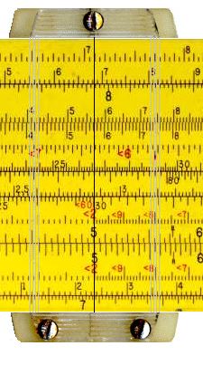
Let’s look at the standard slide rule. You can find a working virtual model here. (The model doesn’t work on an iPad; you’ll have to use it on a computer.) This It is called a 10-inch slide rule because the scales are 10 inches long.

You can move the slide (center section) with your mouse. You can also move the piece withthe screws top and bottom, called the cursor. The cursor is used to read non-adjacent scales and scales on the other side. (Click in the upper right to see the other side). In a real slide rule the slide can be turned over and used with the other side if necessary.

The slide rule only gives the digits of the answer. The decimal point must be determined separately.

The main scales are the C and D scales. These scales are identical and are marked so that the distance from the left end is the mantissa of the common (base 10) logarithm of the number on the scale. The mantissa is the decimal part of the logarithm. The numbers on the C and D scales are all between 0  (= log (1)) and 1 (= log(10)). The scales allow for 3-digit accuracy on the left up to 4 where the spacing allows for only 2-digits. In each case an extra digit may be estimated.

To multiply: slide the 1 on the C scale until it is above the first factor on the D scale. Then find the second factor on the C scale and the number below it on the D scale is the product. Figure 1 shows the computation of 4 x 2 = 8. Remember the distance from the ends are really logarithms, so what you are really doing is log (4) + log (2) = log (4 X 2) = log (8).

Figure 1: Showing 4 x 2 = 8

Other products may also be seen such as 4 x 1.5 = 6, or 40 x 17.5 = 700, etc.

If the second factor is off the right end of the scale; put the 1 on the right side of the C scale over the first factor and the product will be under the second factor. The second figure shows 4 x 5 = 20 (and other products with 4 as a factor). Remember you need to properly place the decimal point.

Figure 2: Showing 4 x 5 = 20

Division is just the reverse: 8 divided by 2 is done by putting the 2 over the 8 and reading the quotient, 4, under the 1 on the C scale. (See figure 1 again). The scales are interchangeable so you could also put the 8 over the 2 (looks better) and find the quotient on the C scale over the 1 on the D scale. Can you find 60 divided by 15 = 4? On figure 2 you can see 2 divided by 5 = 0.4 or 2800 divided by 0.07 = 40,000.

Chain computations can be done by using the cursor to mark (without reading) one answer and then move on to the next, either multiplying or dividing.

The other scales give other functions. The lower scale marked with a radical sign gives square roots. Move the cursor to 2 and read the square root of two (1.414) on the top part of the scale and the square root of 20 (4.472) on the lower part.

Figure 3: Showing \displaystyle \sqrt{2}\approx 1.414 or \displaystyle \sqrt{{20}}\approx 4.47

The S scale gives the sines and cosines of numbers in degrees. Reading from the left the black numbers are for sines and reading from the right the red numbers are for cosines. See figure 3. The cursor is on 60/30 for the sin(30) = cos(60) the value is on the C scale 0.5 (remember you need to supply the decimal). Reading in the other direction the sin-1(0.5) = 30 or cos-1(0.5) = 60.

Figure 4: Showing sin(30) = 0.5 = cos(60) or arcsin(0.5) = 30 or arccos(0.5) = 60.

The CF and DF scales are “folded” at \displaystyle \pi to make multiplying by \displaystyle \pi easier. Computations are done the same way. The CI, DI, CIF, and DIF give the reciprocal (I for inverse) and are read right to left.  T is for tangents a double scale from 0 to 45 degrees on the top and 45 degrees on up at the bottom. I’ll leave the others for you to research.

So, that’s today’s history lesson. Next week, the Spiral Slide Rule – a little more complicated, but a lot more accurate.

Spiral Slide Rule


A Lesson on Sequences

This blog post describes a lesson that investigates some ideas about sequences that are not stressed in the AP Calculus curriculum. The lesson could be an introduction to sequences. I think the lesson would work in an Algebra I course and is certainly suitable for a pre-calculus course. The investigation is of irrational numbers and their decimal representation. The successive decimal approximations to the square root of 2 is an example of a non-decreasing sequence that is bounded above and therefore converges.

Students do not need to know any of that as it will be developed in the lesson. Specifically, don’t even mention square roots, the square root of 2, or even irrational numbers until a student mention something of the sort.

This is not an efficient algorithm for finding square roots. There are far more efficient ways.

We begin with some preliminaries.

Preliminaries

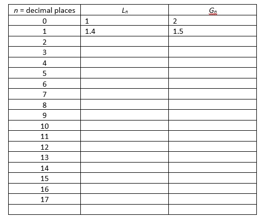
  • There is a blank table that you can copy for students to use here.
  • There is a summary of the new terms used and completed table Sequence Notes. Do not give this out until after the lesson is completed.
  • We will be working with some rather long decimal numbers that will need to be squared. Scientific and graphing calculators usually compute with 14 digits and give their results rounded to 12 digits. Since ours will quickly get longer than that, I suggest you use WolframAlpha. This can be used with a computer online (at wolframalpha.com) or with an app available for smart phones and tablets. It is best if students have this website or app for their individual use.

Students will enter their numbers as shown below. Specifying “30 digits” will produces answers long enough for our purpose. To speed things up, students can edit the current number by changing the last digit in the entry line. When you get started you may have to show students how to do this. Students will need internet access.

  Computer                                                                                 Smart phone

The Lesson

The style of the lesson is Socratic. You, the teacher, will present the problem, explain how they are to go about it, and ask leading questions as appropriate. Some questions are suggested; be ready to ask others.  Later, you will have to explain (define) some new words, but as much as possible let the class suggest what to do. Drag things out of them, rather than telling them.

To begin – Produce some data

Explain to the class that they are going to generate and investigate two lists of numbers (technically called sequences). Each new member of the lists will be a number with one more decimal place than the preceding number.

The first list, whose members are called Ln, will be the largest number with the given number of decimal places, n, whose square is less than two. The subscript, n, stands for the number of decimal places in the number.

Ask: “What is the largest integer whose square is less than 2?” Answer 1, so, L0 = 1. Ask: What is the largest one place decimal whose square is less than 2?”  Answer L1 =1.4.

The second list, Gn, will be the smallest number whose square is greater than 2. So, G0 = 2 and G1 = 1.5. Notice that 1.42 = 1.96 < 2 and 1.52 = 2.25 > 2

Divide the class into 10 groups named Group 0, Group 1, Group 2, …, Group 9. In each round the groups will append their “name” to the preceding decimal and square the resulting number. Group 0 squares 1.40, group 1, squares 1.41, group 2 squares 1.42, etc. using WolframAlpha.

Ask which groups have squares less than two and enter the largest in Ln, the next number will be the smallest number whose square is greater than 2; enter it in Gn.

Complete the table by entering the largest number whose square is less than 2 in the Ln column and the smallest number whose square is greater than 2 in the Gn column. At each stage, each group appends their digit to the most recent Ln . Project or write the table on the board. Students may fill in their own copy. A completed table is here: Sequence Notes and definitions

Next – Lead a discussion

When the table is complete, prompt the students to examine the lists and come up with anything and everything they observe whether it seems important or not. Accept and discuss each observation and let the others say what they think about each observation. (Obviously, don’t deprecate or laugh at any answer – after all at this point, we don’t know what is and is not significant.)

There are (at least) three observations that are significant to what we will consider next. Hopefully, someone will mention them; keep questioning them until they do. They are these, although students may use other terms:

  1. Ln is non-decreasing. Students may first say Ln is increasing. Pause if they do and look at L12 and L13, and L15 and L16. Ask how they know Ln is non-decreasing (because each time we add a digit on the end, you get a bigger number).
  2. Likewise, Gn is non-increasing.
  3. For all n, Ln < Gn, and the numbers differ only in the last digit, and with the last digits differing by 1.

Direct instruction: Explain these ideas and terms (definition)

  • A sequence is a list or set of numbers in a given order.
  • A sequence is bounded above if there exists a number greater than or equal to all the terms of the sequence. The smallest upper bound of a sequence is called its least upper bound (l.u.b.)
  • A sequence is bounded below if there exists a number less than or equal to all the terms of the sequence. The largest lower bound is called the greatest lower bound (g.l.b.)

More questions: Apply these terms to the sequence Ln with questions like these:

  • Is Ln bounded above, below, or not bounded? (Bounded above)
  • Give an example of a number greater than all the terms of Ln. (Many answers: 1,000,000, 4, 2, 1.415, etc. and, in fact, any and every number in Gn)
  • What is the l.u.b. of Ln? Can you think of the smallest number that is an upper bound of this sequence? (Yes, \sqrt{2}. Don’t tell them this – drag it out of them if necessary.) Why? How do you know this?
  • Make the class convince you that for all n, \displaystyle \underset{{n\to \infty }}{\mathop{{\lim }}}\,\left\{ {{{L}_{n}}} \right\}=\sqrt{2}

Ask similar questions about Gn.

  • Is Gn bounded above, below, or not bounded? (Bounded below)
  • Give an example of a number less than all the terms of Ln. (Many answers: any negative number, zero, 1, 1.414, etc. Any and every number in Ln)
  • What is the g.l.b. of Gn? Can you think of the greatest number that is a lower bound of this sequence? (Yes, \sqrt{2}) Why? How do you know this?
  • Make the class convince you that for all n, \displaystyle \underset{{n\to \infty }}{\mathop{{\lim }}}\,\left\{ {{{G}_{n}}} \right\}=\sqrt{2}


Summing Up

Ask, “What’s happening with the numbers in the Ln sequence?” and “What’s happening to the numbers in the Gn sequence?”

The answer you want is that they are getting closer to \sqrt{2}, one from below, the other from above. (As always, wait for a student to suggest this and then let the others discuss it.)

Once everyone is convinced, explain how mathematicians say and write, “gets closer to”:

Mathematicians say that \sqrt{2} is the limiting value (or limit) of both sequences. They write \displaystyle \underset{{n\to \infty }}{\mathop{{\lim }}}\,\left\{ {{{L}_{n}}} \right\}=\sqrt{2} and \displaystyle \underset{{n\to \infty }}{\mathop{{\lim }}}\,\left\{ {{{G}_{n}}} \right\}=\sqrt{2}.

Explain very carefully that while n\to \infty is read, “n approaches infinity,” that infinity, \infty , is not a number. The symbol n\to \infty means that n gets larger without bound or that n gets larger than all (any, every) positive numbers.

In a more technical sense there is an infinite series \displaystyle \sum\limits_{{n=0}}^{\infty }{{{{a}_{n}}\cdot {{{10}}^{{-n}}}}} where \displaystyle {{a}_{n}} is one of the digits 0, 1, 2, 3, …, 9, but there is no formula for listing the values of \displaystyle {{a}_{n}}. However, the sequence of partial sum of this series is the sequence \displaystyle \left\{ {{{L}_{n}}} \right\} which converges to \displaystyle \sqrt{2}. Therefore, \displaystyle \sum\limits_{{n=0}}^{\infty }{{{{a}_{n}}\cdot {{{10}}^{{-n}}}=\sqrt{2}}}

\displaystyle \sqrt{2} is an Irrational number, but this same procedure may be used to find decimal approximation of roots of rational numbers as well. However, for Rational numbers, there are easier ways.

Finally, Irrational numbers are exactly those that cannot be written as repeating (or terminating) decimals. They “go on forever” with no pattern. The decimals you can calculate eventually stop and are rounded to the last digit. Even WolframAlpha and similar computers must eventually do this. Irrational numbers are the limits of sequences like the one we looked at today.

Exercises

  1. Follow the procedure above to find the sequence whose limit is \sqrt{{\frac{{16}}{{121}}}} . Find this number the usual way (simplify and use long division) and compare the results.
  2. Follow the procedure above to find the sequence whose limit is \sqrt{{0.390625}} . Find this number the usual way and compare the results.
  3. Using WolframAlpha determine if the computer is using Ln, Gn. both, or neither when it gives a value for \sqrt{2}. (Hint: enter “square root 2 to 5 digits” and change to 6, 7, and 8 digits; compare the answer with the sequences, you found.)

Answers:

  1. 0.363636…
  2. 0.625
  3. For n = 5 and 6 the numbers are from Ln, for n = 7 and 8 they are from Gn. WolframAlpha is using a different algorithm to compute the square root of 2; the numbers appear from both sequences due to the rounding of the answers. To see WolframAlpha’s algorithm type “square root algorithm” on the entry line. This method also produces a sequence of approximations a/b.

Revised July 28, 2021


AP Calculus Prerequisites

College Board Prerequisites

Whenever I led a calculus workshop or APSI, I always spent a little time discussing the prerequisites for AP Calculus. Unfortunately, in some schools AP Calculus is a course for only the talented and little time is spent aligning the mathematics program and courses from 7th grade on so that more students will be able to take AP Calculus. But a program that includes the prerequisite for calculus will be a good program because of this. Such a program will also benefit students who do not take AP Calculus, but still need a good mathematics program for when they attend college.

Teachers in the earlier courses are usually appreciative of guidance from the AP Calculus teacher as to what should be included to prepare students for calculus. This is part of the rationale of the AP’s math Vertical Team program.

Below in blue is the entire prerequisite paragraph from the 2019 AP Calculus Course and Exam Description p. 7. I have separated the parts and commented on each.

Before studying calculus, all students should complete the equivalent of four years of secondary mathematics designed for college-bound students:

The four years is needed. Students should not be rushed.

In some respects, this is a political statement: four years means starting in 8th grade or earlier. While some of the most talented students can probably catch up by doing two years in one or three years in two, this is not the usual case. Learning math thoroughly takes four years.

Once in my district, our junior high decided to raise the standards for their “advanced” course that taught Algebra I in 8th grade. No one told us, so the next year we found only one class, instead of two, that could be ready for AP Calculus by the time they were seniors. We tried a three-years-in-two approach. It met with only limited success. Algebra I in 8th grade is required and really should be for everyone otherwise you are denying students the chance to even consider AP Calculus when they are seniors.

 courses that should prepare them with a strong foundation in reasoning with algebraic symbols and working with algebraic structures.

Using and understanding the use of mathematical notation is a must. Throughout the four years, algebra and its structure should be emphasized.  So, it’s not just 4 years of math, but four years of a good algebra-based math program. But algebra is not the only thing:

Prospective calculus students should take courses in which they study algebra, geometry, trigonometry, analytic geometry, and elementary functions.

All these courses are related and lead to a fuller understanding of high school math topics.

These functions include linear, polynomial, rational, exponential, logarithmic, trigonometric, inverse trigonometric, and piecewise-defined functions.

This is a list of the types of functions that should be included. They are the basic functions studied in the calculus. Linear and simple polynomial functions start in Algebra I and the others are added later. Piecewise-define functions also start early – the absolute value function is a piecewise-defined function.

In particular, before studying calculus, students must be familiar with the properties of functions, the composition of functions, the algebra of functions, and the graphs of functions.

The algebra of functions means learning how to add, subtract, multiply, divide, and compose functions and how doing so affects the properties and graphs of the resulting functions. The graphs of these functions and how doing algebra, composition, and transformations affects the graph is important.

Students must also understand the language of functions (domain and range, odd and even, periodic, symmetry, zeros, intercepts, and descriptors such as increasing and decreasing).

The list of the language functions is too short. Some terms such as increasing, decreasing, maximum and minimum values, concavity and others often considered the province of calculus all come up in the study of functions and can and should be discussed when they arise using the correct terminology and notation. There is no need to wait for calculus to use them to describe functions, graphs and transformations. An informal use and understanding of continuity and limits should be included. Asymptotes should not be overlooked (they are the graphical manifestation of limits and continuity or the lack of same). The more students learn before calculus, the less you’ll have to do in calculus.

Students should also know how the sine and cosine functions are defined from the unit circle and know the values of the trigonometric functions at the numbers 0,\tfrac{\pi }{6},\tfrac{\pi }{4},\tfrac{\pi }{3},\tfrac{\pi }{2} and their multiples.

Yes, with all the technology available these basic trig facts should be learned (learned, not just memorized); they are always tested on the AP Exams.

Students who take AP Calculus BC should have basic familiarity with sequences and series, as well as some exposure to parametric and polar equations.

Here I disagree. Parametric equations, vector equations and polar equations should be a part of the curriculum for all students. Students who do not take BC calculus, may well take more math courses in college and should understand these ways of working with the plane and with functions defined in different ways.


This list does not define the entire high school math program. There are other topics that can and probably should be included – statistics, systems of equations, linear algebra and matrices, proofs, probability to name a few. What it does define is what should be included so that students will be ready for calculus.

What I think is missing here is the use of technology. In the world today mathematics is done with technology. The proper use of technology should be an integral part of the program from before Algebra I.

AP Statistics is a great course. Students who have completed Algebra II should consider this course. However, AP Statistics it is not an algebra-based course. About three-quarters of the course and its exam is writing; there is very little algebra involved. Therefore, students should not be taking AP Statistics instead of AP Calculus, or if they are not taking calculus, instead of a third year of Algebra. The AP Statistic prerequisites state:

Students who wish to leave open the option of taking calculus in college should include precalculus [i.e. a third year of algebra] in their high school program and perhaps take AP Statistics concurrently with precalculus.

Students with the appropriate mathematical background are encouraged to take both AP Statistics and AP Calculus in high school.

AP Statistics 2019 Course and Exam Description p. 7, emphasis added.

The point is that students should not have a year in high school without an algebra course. A year in which to forget their algebra before going to college where they may need it again is not a good idea.


I like to think of all the mathematics courses before calculus as “precalculus.” In many schools, “precalculus” is the name of the last course before calculus. That’s okay, I guess. What I disagree with is that often the precalculus teacher, with the good intention of preparing their students for calculus, teaches them “derivatives.” By which they mean the rules for computing derivatives. This really does not help the students or the calculus teacher.

Derivatives are limits and derivatives are slopes; computing derivatives is the least of your worries. If students have learned all the other precalculus topics (including parametric, vector, and polar equations) well and there is time left, consider delving further into limits and continuity. Limits seem to be more difficult to understand and some repeating of the topic when students arrive in calculus will do no harm. Leave the calculus for the calculus class. (The exception is when the precalculus class is intentionally meant to get an early start on the calculus; when it is taught by the calculus teacher or a teacher who is aware of the Essential Knowledge and Learning objective of the AP Calculus course.)  – Just my opinion.


High School Prerequisites

Some high schools add their own prerequisites to enter AP Calculus courses. This usually means students have to earn a significantly higher score than just a passing grade in the precalculus course(s). I do not agree with such a policy.  It excludes students who may benefit. If your student passed the precalculus course, even with a low grade, how can you say they are not ready for calculus? What will make them more ready? True, they may have to struggle, but that won’t hurt them. You may want to council them (and their parents) and explain, without discouraging them, the amount of work and time required in a college level course like AP. Explain the amount of time and work they will have to spend once they get to college in a course that meets far fewer times then AP Calculus to cover the same material. Even if they end up without earning a qualifying score on the AP Exam, they will still benefit by putting in the time and effort. If they want to try, encourage them.


Polar Equations

Ideally, as with parametric and vector functions, polar curves should be introduced and covered thoroughly in a pre-calculus course. Questions on the BC exams have been concerned with calculus ideas related to polar curves. Students have not been asked to know the names of the various curves (rose, curves, limaçons, etc.). The graphs are usually given in the stem of the problem, but students should know how to graph polar curves on their calculator, and the simplest by hand.

What students should know how to do:

  • Calculate the coordinates of a point on the graph,
  • Find the intersection of two graphs (to use as limits of integration).
  • Find the area enclosed by a graph or graphs: Area =\displaystyle A=\tfrac{1}{2}\int_{{{\theta }_{1}}}^{{{\theta }_{2}}}{(r(}θ\displaystyle ){{)}^{2}}dθ
  • Use the formulas x\left( \theta  \right)\text{ }=~r\left( \theta  \right)\text{cos}\left( \theta  \right)~~\text{and}~y\left( \theta  \right)\text{ }=~r(\theta )\text{sin}\left( \theta  \right)~  to convert from polar to parametric form,
  • Calculate \displaystyle \frac{dy}{d\theta } and \displaystyle \frac{dx}{d\theta } (Hint: use the product rule on the equations in the previous bullet).
  • Discuss the motion of a particle moving on the graph by discussing the meaning of \displaystyle \frac{dr}{d\theta } (motion towards or away from the pole), \displaystyle \frac{dy}{d\theta } (motion in the vertical direction) or \displaystyle \frac{dx}{d\theta } (motion in the horizontal direction).
  • Find the slope at a point on the graph, \displaystyle \frac{dy}{dx}=\frac{dy/d\theta }{dx/d\theta }.

This topic appears only occasionally on the free-response section of the exam instead of the Parametric/vector motion question. The most recent on the released exams were in 2007,  2013, 2014, and 2017. If the topic is not on the free-response then 1, or maybe 2 questions, probably finding area, can be expected on the multiple-choice section.

Shorter questions on these ideas appear in the multiple-choice sections. As always, look over as many questions of this kind from past exams as you can find.


Here are the few post I have written on polar curves and polar graphing.

Limaçons   A discussion of how polar curves are graphed

Back in the summer of 2014 I got interested in some polar equations and wrote a series of post on them which include some gifs showing how they are graphed. They are nothing that will appear on the AP exams. You can use them as enrichment if you like.

Rolling Circles

Roulettes and Calculus

Epitrochoids

Epicycloids

Hypocycloids and Hypotrochoids

Roulettes and Art – 1  

Roulettes and Art – 2