Unit 8 – Applications of Integration

I haven’t missed Unit 7! This unit seems to fit more logically after the opening unit on integration (Unit 6). The Course and Exam Description (CED) places Unit 7 Differential Equations before Unit 8 probably because the previous unit ended with techniques of antidifferentiation. My guess is that many teachers will teach Unit 8: Applications of Integration immediately after Unit 6 and before Unit 7: Differential Equations. The order is up to you. Unit 7 will post next Tuesday.

Unit 8 includes some standard problems solvable by integration (CED – 2019 p. 143 – 161). These topics account for about 10 – 15% of questions on the AB exam and 6 – 9% of the BC questions.

Topics 8.1 – 8.3 Average Value and Accumulation

Topic 8.1 Finding the Average Value of a Function on an Interval Be sure to distinguish between average value of a function on an interval, average rate of change on an interval and the mean value

Topic 8.2 Connecting Position, Velocity, and Acceleration of Functions using Integrals Distinguish between displacement (= integral of velocity) and total distance traveled (= integral of speed)

Topic 8. 3 Using Accumulation Functions and Definite Integrals in Applied Contexts The integral of a rate of change equals the net amount of change. A really big idea and one that is tested on all the exams. So, if you are asked for an amount, look around for a rate to integrate.

Topics 8.4 – 8.6 Area

Topic 8.4 Finding the Area Between Curves Expressed as Functions of x

Topic 8.5 Finding the Area Between Curves Expressed as Functions of y

Topic 8.6 Finding the Area Between Curves That Intersect at More Than Two Points Use two or more integrals or integrate the absolute value of the difference of the two functions. The latter is especially useful when do the computation of a graphing calculator.

Topics 8.7 – 8.12 Volume

Topic 8.7 Volumes with Cross Sections: Squares and Rectangles

Topic 8.8 Volumes with Cross Sections: Triangles and Semicircles

Topic 8.9 Volume with Disk Method: Revolving around the x– or y-Axis Volumes of revolution are volumes with circular cross sections, so this continues the previous two topics.

Topic 8.10 Volume with Disk Method: Revolving Around Other Axes

Topic 8.11 Volume with Washer Method: Revolving Around the x– or y-Axis See Subtract the Hole from the Whole for an easier way to remember how to do these problems.

Topic 8.12 Volume with Washer Method: Revolving Around Other Axes. See Subtract the Hole from the Whole for an easier way to remember how to do these problems.

Topic 8.13  Arc Length BC Only

Topic 8.13 The Arc Length of a Smooth, Planar Curve and Distance Traveled  BC ONLY


Timing

The suggested time for Unit 8 is  19 – 20 classes for AB and 13 – 14 for BC of 40 – 50-minute class periods, this includes time for testing etc.


Previous posts on these topics for both AB and BC include:

Average Value and Accumulation

Average Value of a Function and 

Most Triangles Are Obtuse!

Half-full or Half-empty

Accumulation: Need an Amount?

AP Accumulation Questions

Good Question 7 – 2009 AB 3 Accumulation, explain the meaning of an integral in context, unit analysis

Good Question 8 – or Not Unit analysis

Graphing with Accumulation 1 Seeing increasing and decreasing through integration

Graphing with Accumulation 2 Seeing concavity through integration

Adapting AB 1 / BC 1

Area

Area Between Curves

Under is a Long Way Down  Avoiding “negative area.”

Improper Integrals and Proper Areas  BC Topic

Math vs. the “Real World”  Improper integrals  BC Topic

Adapting 2021 AB 3 / BC 3

Volume

Volumes of Solids with Regular Cross-sections

Volumes of Revolution

Why You Never Need Cylindrical Shells

Visualizing Solid Figures 1

Visualizing Solid Figures 2

Visualizing Solid Figures 3

Visualizing Solid Figures 4

Visualizing Solid Figures 5

Painting a Point

Subtract the Hole from the Whole and Does Simplifying Make Things Simpler?

Adapting 2021 AB 3 / BC 3

Other Applications of Integrals

Density Functions have been tested in the past, but are not specifically listed on the CED then or now.

Who’d a Thunk It? Some integration problems suitable for graphing calculator solution


Here are links to the full list of posts discussing the ten units in the 2019 Course and Exam Description.

2019 CED – Unit 1: Limits and Continuity

2019 CED – Unit 2: Differentiation: Definition and Fundamental Properties.

2019 CED – Unit 3: Differentiation: Composite , Implicit, and Inverse Functions

2019 CED – Unit 4 Contextual Applications of the Derivative  Consider teaching Unit 5 before Unit 4

2019 – CED Unit 5 Analytical Applications of Differentiation  Consider teaching Unit 5 before Unit 4

2019 – CED Unit 6 Integration and Accumulation of Change

2019 – CED Unit 7 Differential Equations  Consider teaching after Unit 8

2019 – CED Unit 8 Applications of Integration   Consider teaching after Unit 6, before Unit 7

2019 – CED Unit 9 Parametric Equations, Polar Coordinates, and Vector-Values Functions 

2019 CED Unit 10 Infinite Sequences and Series


Advertisement

Unit 6 – Integration and Accumulation of Change

Unit 6 develops the ideas behind integration, the Fundamental Theorem of Calculus, and Accumulation. (CED – 2019 p. 109 – 128). These topics account for about 17 – 20% of questions on the AB exam and 17 – 20% of the BC questions.

Topics 6.1 – 6.4 Working up to the FTC

Topic 6.1 Exploring Accumulations of Change Accumulation is introduced through finding the area between the graph of a function and the x-axis. Positive and negative rates of change, unit analysis.

Topic 6.2 Approximating Areas with Riemann Sums Left-, right-, midpoint Riemann sums, and Trapezoidal sums, with uniform partitions are developed. Approximating with numerical methods, including use of technology are considered. Determining if the approximation is an over- or under-approximation.

Topic 6.3 Riemann Sums, Summation Notation and the Definite Integral. The definition integral is defined as the limit of a Riemann sum.

Topic 6.4 The Fundamental Theorem of Calculus (FTC) and Accumulation Functions Functions defined by definite integrals and the FTC.

Topic 6.5 Interpreting the Behavior of Accumulation Functions Involving Area Graphical, numerical, analytical, and verbal representations.

Topic 6.6 Applying Properties of Definite Integrals Using the properties to ease evaluation, evaluating by geometry and dealing with discontinuities.

Topic 6.7 The Fundamental Theorem of Calculus and Definite Integrals Antiderivatives. (Note: I suggest writing the FTC in this form displaystyle int_{a}^{b}{{{f}'left( x right)}}dx=fleft( b right)-fleft( a right) because it seem more efficient then using upper case and lower case f.)

Topics 6.5 – 6.14 Techniques of Integration

Topic 6.8 Finding Antiderivatives and Indefinite Integrals: Basic Rules and Notation. Using basic differentiation formulas to find antiderivatives. Some functions do not have closed-form antiderivatives. (Note: While textbooks often consider antidifferentiation before any work with integration, this seems like the place to introduce them. After learning the FTC students have a reason to find antiderivatives. See Integration Itinerary

Topic 6.9 Integration Using Substitution The u-substitution method. Changing the limits of integration when substituting.

Topic 6.10 Integrating Functions Using Long Division and Completing the Square 

Topic 6.11 Integrating Using Integration by Parts (BC ONLY)

Topic 6.12 Integrating Using Linear Partial Fractions (BC ONLY)

Topic 6.13 Evaluating Improper Integrals (BC ONLY) Showing the work requires students to show correct limit notation.

Topic 6.14 Selecting Techniques for Antidifferentiation This means practice, practice, practice.


Timing

The suggested time for Unit 6 is  18 – 20 classes for AB and 15 – 16 for BC of 40 – 50-minute class periods, this includes time for testing etc.


Previous posts on these topics include:

Introducing Integration

Integration Itinerary

The Old Pump and Flying to Integrationland   Two introductory explorations

Working Towards Riemann Sums

Riemann Sums

The Definition of the Definite Integral

Foreshadowing the FTC 

The Fundamental Theorem of Calculus

More About the FTC

Y the FTC?

Area Between Curves

Under is a Long Way Down 

Properties of Integrals 

Trapezoids – Ancient and Modern  On Trapezoid sums

Good Question 9 – Riemann Reversed   Given a Riemann sum can you find the Integral it converges to?  A common and difficult AP Exam problem

Adapting 2021 AB 1 / BC 1

Adapting 2021 AB 4 / BC 4

Accumulation

Accumulation: Need an Amount?

Good Question 7 – 2009 AB 3

Good Question 8 – or Not?  Unit analysis

AP Exams Accumulation Question    A summary of accumulation ideas.

Graphing with Accumulation 1

Graphing with Accumulation 2

Accumulation and Differential Equations 

Painting a Point

Techniques of Integrations (AB and BC)

Antidifferentiation

Why Muss with the “+C”?

Good Question 13  More than one way to skin a cat.

Integration by Parts – a BC Topic

Integration by Parts 1

Integration by Part 2

Parts and More Parts

Good Question 12 – Parts with a Constant?

Modified Tabular Integration 

Improper Integrals and Proper Areas

Math vs the Real World Why displaystyle int_{{-infty }}^{infty }{{frac{1}{x}}}dx does not converge.


Here are links to the full list of posts discussing the ten units in the 2019 Course and Exam Description.

2019 CED – Unit 1: Limits and Continuity

2019 CED – Unit 2: Differentiation: Definition and Fundamental Properties.

2019 CED – Unit 3: Differentiation: Composite , Implicit, and Inverse Functions

2019 CED – Unit 4 Contextual Applications of the Derivative  Consider teaching Unit 5 before Unit 4

2019 – CED Unit 5 Analytical Applications of Differentiation  Consider teaching Unit 5 before Unit 4

2019 – CED Unit 6 Integration and Accumulation of Change

2019 – CED Unit 7 Differential Equations  Consider teaching after Unit 8

2019 – CED Unit 8 Applications of Integration   Consider teaching after Unit 6, before Unit 7

2019 – CED Unit 9 Parametric Equations, Polar Coordinates, and Vector-Values Functions 

2019 CED Unit 10 Infinite Sequences and Series


Applications of Integration – Unit 8

I haven’t missed Unit 7! This unit seems to fit more logically after the opening unit on integration (Unit 6). The Course and Exam Description (CED) places Unit 7 Differential Equations before Unit 8 probably because the previous unit ended with techniques of antidifferentiation. My guess is that many teachers will teach Unit 8: Applications of Integration immediately after Unit 6 and before Unit 7: Differential Equations. The order is up to you. Unit 7 will post next Tuesday.

Unit 8 includes some standard problems solvable by integration (CED – 2019 p. 143 – 161). These topics account for about 10 – 15% of questions on the AB exam and 6 – 9% of the BC questions.

Topics 8.1 – 8.3 Average Value and Accumulation

Topic 8.1 Finding the Average Value of a Function on an Interval Be sure to distinguish between average value of a function on an interval, average rate of change on an interval and the mean value

Topic 8.2 Connecting Position, Velocity, and Acceleration of Functions using Integrals Distinguish between displacement (= integral of velocity) and total distance traveled (= integral of speed)

Topic 8. 3 Using Accumulation Functions and Definite Integrals in Applied Contexts The integral of a rate of change equals the net amount of change. A really big idea and one that is tested on all the exams. So, if you are asked for an amount, look around for a rate to integrate.

Topics 8.4 – 8.6 Area

Topic 8.4 Finding the Area Between Curves Expressed as Functions of x

Topic 8.5 Finding the Area Between Curves Expressed as Functions of y

Topic 8.6 Finding the Area Between Curves That Intersect at More Than Two Points Use two or more integrals or integrate the absolute value of the difference of the two functions. The latter is especially useful when do the computation of a graphing calculator.

Topics 8.7 – 8.12 Volume

Topic 8.7 Volumes with Cross Sections: Squares and Rectangles

Topic 8.8 Volumes with Cross Sections: Triangles and Semicircles

Topic 8.9 Volume with Disk Method: Revolving around the x– or y-Axis Volumes of revolution are volumes with circular cross sections, so this continues the previous two topics.

Topic 8.10 Volume with Disk Method: Revolving Around Other Axes

Topic 8.11 Volume with Washer Method: Revolving Around the x– or y-Axis See Subtract the Hole from the Whole for an easier way to remember how to do these problems.

Topic 8.12 Volume with Washer Method: Revolving Around Other Axes. See Subtract the Hole from the Whole for an easier way to remember how to do these problems.

Topic 8.13  Arc Length BC Only

Topic 8.13 The Arc Length of a Smooth, Planar Curve and Distance Traveled  BC ONLY


Timing

The suggested time for Unit 8 is  19 – 20 classes for AB and 13 – 14 for BC of 40 – 50-minute class periods, this includes time for testing etc.


Previous posts on these topics for both AB and BC include:

Average Value and Accumulation

Average Value of a Function and Average Value of a Function

Half-full or Half-empty

Accumulation: Need an Amount?

AP Accumulation Questions

Good Question 7 – 2009 AB 3 Accumulation, explain the meaning of an integral in context, unit analysis

Good Question 8 – or Not Unit analysis

Graphing with Accumulation 1 Seeing increasing and decreasing through integration

Graphing with Accumulation 2 Seeing concavity through integration

Area

Area Between Curves

Under is a Long Way Down  Avoiding “negative area.”

Improper Integrals and Proper Areas  BC Topic

Math vs. the “Real World”  Improper integrals  BC Topic

Volume

Volumes of Solids with Regular Cross-sections

Volumes of Revolution

Why You Never Need Cylindrical Shells

Visualizing Solid Figures 1

Visualizing Solid Figures 2

Visualizing Solid Figures 3

Visualizing Solid Figures 4

Visualizing Solid Figures 5

Painting a Point

Subtract the Hole from the Whole and Does Simplifying Make Things Simpler?

Other Applications of Integrals

Density Functions have been tested in the past, but are not specifically listed on the CED then or now.

Who’d a Thunk It? Some integration problems suitable for graphing calculator solution


Here are links to the full list of posts discussing the ten units in the 2019 Course and Exam Description.

2019 CED – Unit 1: Limits and Continuity

2019 CED – Unit 2: Differentiation: Definition and Fundamental Properties.

2019 CED – Unit 3: Differentiation: Composite , Implicit, and Inverse Functions

2019 CED – Unit 4 Contextual Applications of the Derivative  Consider teaching Unit 5 before Unit 4

2019 – CED Unit 5 Analytical Applications of Differentiation  Consider teaching Unit 5 before Unit 4

2019 – CED Unit 6 Integration and Accumulation of Change

2019 – CED Unit 7 Differential Equations  Consider teaching after Unit 8

2019 – CED Unit 8 Applications of Integration   Consider teaching after Unit 6, before Unit 7

2019 – CED Unit 9 Parametric Equations, Polar Coordinates, and Vector-Values Functions 

2019 CED Unit 10 Infinite Sequences and Series


Integration and Accumulation of Change – Unit 6

Unit 6 develops the ideas behind integration, the Fundamental Theorem of Calculus, and Accumulation. (CED – 2019 p. 109 – 128 ). These topics account for about 17 – 20% of questions on the AB exam and 17 – 20% of the BC questions.

Topics 6.1 – 6.4 Working up to the FTC

Topic 6.1 Exploring Accumulations of Change Accumulation is introduced through finding the area between the graph of a function and the x-axis. Positive and negative rates of change, unit analysis.

Topic 6.2 Approximating Areas with Riemann Sums Left-, right-, midpoint Riemann sums, and Trapezoidal sums, with uniform partitions are developed. Approximating with numerical methods, including use of technology are considered. Determining if the approximation is an over- or under-approximation.

Topic 6.3 Riemann Sums, Summation Notation and the Definite Integral. The definition integral is defined as the limit of a Riemann sum.

Topic 6.4 The Fundamental Theorem of Calculus (FTC) and Accumulation Functions Functions defined by definite integrals and the FTC.

Topic 6.5 Interpreting the Behavior of Accumulation Functions Involving Area Graphical, numerical, analytical, and verbal representations.

Topic 6.6 Applying Properties of Definite Integrals Using the properties to ease evaluation, evaluating by geometry and dealing with discontinuities.

Topic 6.7 The Fundamental Theorem of Calculus and Definite Integrals  Antiderivatives. (Note: I suggest writing the FTC in this form \displaystyle \int_{a}^{b}{{{f}'\left( x \right)}}dx=f\left( b \right)-f\left( a \right) because it seem more efficient then using upper case and lower case f.)

Topics 6.5 – 6.14 Techniques of Integration

Topic 6.8 Finding Antiderivatives and Indefinite Integrals: Basic Rules and Notation. Using basic differentiation formulas to find antiderivatives. Some functions do not have closed-form antiderivatives. (Note: While textbooks often consider antidifferentiation before any work with integration, this seems like the place to introduce them. After learning the FTC students have a reason to find antiderivatives. See Integration Itinerary

Topic 6.9 Integration Using Substitution The u-substitution method. Changing the limits of integration when substituting.

Topic 6.10 Integrating Functions Using Long Division and Completing the Square 

Topic 6.11 Integrating Using Integration by Parts  (BC ONLY)

Topic 6.12 Integrating Using Linear Partial Fractions  (BC ONLY)

Topic 6.13 Evaluating Improper Integrals (BC ONLY) Showing the work requires students to show correct limit notation.

Topic 6.14 Selecting Techniques for Antidifferentiation This means practice, practice, practice.


Timing

The suggested time for Unit 6 is  18 – 20 classes for AB and 15 – 16 for BC of 40 – 50-minute class periods, this includes time for testing etc.


Previous posts on these topics include:

Introducing Integration

Integration Itinerary

The Old Pump and Flying to Integrationland   Two introductory explorations

Working Towards Riemann Sums

Riemann Sums

The Definition of the Definite Integral

Foreshadowing the FTC 

The Fundamental Theorem of Calculus

More About the FTC

Y the FTC?

Area Between Curves

Under is a Long Way Down 

Properties of Integrals 

Trapezoids – Ancient and Modern  On Trapezoid sums

Good Question 9 – Riemann Reversed   Given a Riemann sum can you find the Integral it converges to?  A common and difficult AP Exam problem

Accumulation

Accumulation: Need an Amount?

Good Question 7 – 2009 AB 3

Good Question 8 – or Not?  Unit analysis

AP Exams Accumulation Question    A summary of accumulation ideas.

Graphing with Accumulation 1

Graphing with Accumulation 2

Accumulation and Differential Equations 

Painting a Point

Techniques of Integrations (AB and BC)

Antidifferentiation

Why Muss with the “+C”?

Good Question 13  More than one way to skin a cat.

Integration by Parts – a BC Topic

Integration by Parts 1

Integration by Part 2

Parts and More Parts

Good Question 12 – Parts with a Constant?

Modified Tabular Integration 

Improper Integrals and Proper Areas

Math vs the Real World Why \displaystyle \int_{{-\infty }}^{\infty }{{\frac{1}{x}}}dx does not converge.


Here are links to the full list of posts discussing the ten units in the 2019 Course and Exam Description.

2019 CED – Unit 1: Limits and Continuity

2019 CED – Unit 2: Differentiation: Definition and Fundamental Properties.

2019 CED – Unit 3: Differentiation: Composite , Implicit, and Inverse Functions

2019 CED – Unit 4 Contextual Applications of the Derivative  Consider teaching Unit 5 before Unit 4

2019 – CED Unit 5 Analytical Applications of Differentiation  Consider teaching Unit 5 before Unit 4

2019 – CED Unit 6 Integration and Accumulation of Change

2019 – CED Unit 7 Differential Equations  Consider teaching after Unit 8

2019 – CED Unit 8 Applications of Integration   Consider teaching after Unit 6, before Unit 7

2019 – CED Unit 9 Parametric Equations, Polar Coordinates, and Vector-Values Functions 

2019 CED Unit 10 Infinite Sequences and Series


Good Question 8 – or not?

Seattle rainToday’s question is not a good question. It’s a bad question.

But sometimes a bad question can become a good one.

This one leads first to a discussion of units, then to all sorts of calculus.

Here’s the question a teacher sent me this week taken from his textbook:

The normal monthly rainfall at the Seattle-Tacoma airport can be approximated by the model R=3.121+2.399\sin \left( 0.524t+1.377 \right)
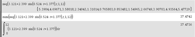
, where R is measured in inches and t is the time in months, t = 1 being January. Use integration to approximate the normal annual rainfall.  Hint: Integrate over the interval [0,12].

Of course, with the hint it’s not difficult to know what to do and that makes it less than a good question right there. The answer is \displaystyle \int_{0}^{12}{R(t)dt=37.4736} 
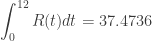
inches. You could quit here and go on to the next question, but …

Then a student asked. “If R is in inches shouldn’t be in units of the integral be inch-months, since the unit of an integral is the unit of the integrand times the units of the independent variable?”  Well, yes, they should. So, what’s up with that?

Also, the teacher figured that the integral of a rate is an amount and our answer is an amount, so why isn’t the integrand a rate?

The only answer I could come up with is that the statement “R is measured in inches” is incorrect; R should be measured in inches /month. The opening phrase “normal monthly rainfall” also seems to point to the correct units for R being inches/month.

Problem solved; or maybe does this lead to a different concern?

The teacher pointed out that R(6) = 0.7658 inches is a reasonable answer for the amount of rain in June whereas \displaystyle \int_{0}^{6}{R(t)dt=}20.4786 is not.

If R is a rate, then the amount of rain that falls in June (t = 6) is given by \displaystyle \int_{5}^{6}{R(t)dt}=0.9890.

From here on we will assume that R is a rate with units of inches/month. Here are the individual monthly rates calculated with a CAS. Ques 8 a

The total amount of rainfall (second line above) appears be R(1) + R(2) + R(3) + … +R(12) = 37.4742. This is very close to the amount calculated by integration.

The slight difference of 0.0006 is not a round off error.

Remember, behind every definite integral there is a Riemann sum!

Again, the units are the problem. Why does the sum of the monthly rates seem to give the total amount?  The reason is that the terms of the sequence above are actually the values of a right-side Riemann sum of the rate, R(t), over the interval [0,12] with 12 equal subdivisions of width 1 (month) each with the 1’s left out as 1’s often are. Therefore, their sum should come close to the total yearly rainfall, but it is really just an approximation of it.

The actual total for any month, n, is given by \displaystyle \int_{n-1}^{n}{r(t)}dt. For example the amount of rain that falls in June is given by \displaystyle \int_{5}^{6}{R(t)dt}=0.9890 inches.

Here is the sequence of the actual monthly rainfall values in inches, and their sum.

Ques 8 b

This agrees with the integral. Why? Because one of  the properties of integrals tell us that \displaystyle \sum\limits_{n=1}^{12}{\int_{n-1}^{n}{r(t)dt}}=\int_{0}^{12}{r(t)dt}.


Another instructive thing with this integral is this: The function R=3.121+2.399\sin \left( 0.524t+1.377 \right) is periodic with a period of  \frac{2\pi }{0.524}\approx 11.9908\approx 12. So the sine function takes on (almost) all its values in a year, as you would expect. Since the sine values all but cancel each other out

\displaystyle \int_{0}^{12}{3.121+2.399\sin \left( 0.524t+1.377 \right)dt}\approx \int_{0}^{12}{3.121dt=3.121\left( 12-0 \right)=37.452}. Close!

The total rainfall divided by 12 is \frac{37.452}{12}=3.121 this must be close to the average rainfall each month. The average rainfall is \displaystyle \frac{1}{12}\int_{0}^{12}{R\left( t \right)dt}=3.1228 inches. Close, again!


So, there you have it. Is this a good question or not? We considered all these concepts while working not just with an equation but with numbers from a poorly stated problem:

  • Reading and interpreting words.
  • Unit analysis
  • Integration by technology
  • Realizing that a pretty good approximation is not correct, due again to units.
  • A Riemann sum approximation in a real situation that comes very close to the value by integration
  • Using a property of a periodic function to greatly simplify an integral
  • Finding average value two ways

So, it turned out to be a sunny day in Seattle.seattle sun

.

Properties of Integrals

In the last two posts we looked at activities that lead to the FTC. Today I would like to build on that activity to demonstrate some of the important properties of integrals. I am never in favor of giving students theorems or properties like these and saying, “Here they are, learn them!” Nor do I think everything has to be done up with a detailed “proof.” So here is an approach between those alternatives.

Look at the activity in the last post where we considered three functions: F1(t) = 3, F2(x) = 2t and F3(t) = 2t + 3. We built new functions that gave the area between these functions and the t-axis. We expressed these as regular looking functions and also as functions defined by definite integrals – integrals where the upper limit of integration was a variable, x. We also made tables of values for these functions. Return to these tables and consider the following properties of integrals.

      1. Integrals are additive. I hope you noticed that F3 = F1 + F2.  Look at the values in the table you made for the area functions, and you will see that \int_{a}^{x}{F1(t)\pm F2(t)dt}=\int_{a}^{x}{F1(t)dt}\pm \int_{a}^{x}{F2(t)dt}. This is important because when evaluating definite integrals this allows us to do them term by term.
      2. Constants may be factored out of the integrand and written in front: \int_{a}^{b}{k\cdot f\left( t \right)}dt=k\cdot \int_{a}^{b}{f\left( t \right)dt} . To see this make a quick table for the area between F(t) = t and compare it to the area functions for F2(t) = 2t.
      3. Previously, we restricted our domain to nonnegative numbers. Let’s change that. Make a table for the three area functions A1(x), A2(x) and A3(x) for x = -1, -2, -3, -4, and -5. Work from the functions you wrote, not from the geometry. What do you notice? There are negative and zero values!  Areas are never negative. How do you explain what’s happened?

        Write the corresponding definite integrals. Be careful, the upper limits are now less than the lower limits. Think of the Riemann sums that are behind the limits. Since x moves left, the values in the Riemann sum will be negative producing negative values for A1(x). In A2(x) both and the function values are negative, producing a positive result. Can you explain what’s going on with A3(x) which has positive, zero and negative values?

        The short answer is that if the upper and the lower limits of integration are switched then the resulting integrals are opposites of each other:\int_{a}^{b}{f\left( x \right)dx}=-\int_{b}^{a}{f\left( x \right)dx}

      4. Next use your graph and geometry to find that area between F3(t) and the t-axis between, say, x = 3 and x =  5, and then use the table value to show that \int_{0}^{3}{F3(t)dt}+\int_{3}^{5}{F3(t)dt}=\int_{0}^{5}{F3(t)dt} . Now use those numbers and the property in paragraph 3 to show that \int_{3}^{5}{F3(t)dt}+\int_{5}^{0}{F3(t)dt}=\int_{3}^{0}{F3(t)dt}.
        In general, \int_{a}^{b}{f\left( x \right)dx}+\int_{b}^{c}{f\left( x \right)dx}=\int_{a}^{c}{f\left( x \right)dx} regardless of the order of a ,b and c. The only thing that matters is that (1) the lower limit in the first integral on the left is the lower limit on the right, (2) the upper limit on the last integral on the left is the upper limit on the right, and (3) on the left the upper limit on one integral is the lower limit on the next. You can even string more integrals together as long as you follow the pattern.
      1. A final property which can be seen by comparing the graphs and the areas between them and the t-axis for F2(x) and F3(x) is this: If f\left( x \right)\le g\left( x \right) on the interval [a, b], then \int_{a}^{b}{f\left( x \right)dx}\le \int_{a}^{b}{g\left( x \right)dx}. This is sometimes called the “Racetrack Principle.” Interpreting f and g as rates and their integrals as amounts (or distances), then in the same interval, the faster horse travels farther.

Happy Holiday. My next post will be Friday December 28, 2012.