Good Question 8 – or not?

Seattle rainToday’s question is not a good question. It’s a bad question.

But sometimes a bad question can become a good one.

This one leads first to a discussion of units, then to all sorts of calculus.

Here’s the question a teacher sent me this week taken from his textbook:

The normal monthly rainfall at the Seattle-Tacoma airport can be approximated by the model R=3.121+2.399\sin \left( 0.524t+1.377 \right), where R is measured in inches and t is the time in months, t = 1 being January. Use integration to approximate the normal annual rainfall.  Hint: Integrate over the interval [0,12].

Of course, with the hint it’s not difficult to know what to do and that makes it less than a good question right there. The answer is \displaystyle \int_{0}^{12}{R(t)dt=37.4736} inches. You could quit here and go on to the next question, but …

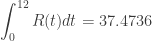
Then a student asked. “If R is in inches shouldn’t be in units of the integral be inch-months, since the unit of an integral is the unit of the integrand times the units of the independent variable?”  Well, yes, they should. So, what’s up with that?

Also, the teacher figured that the integral of a rate is an amount and our answer is an amount, so why isn’t the integrand a rate?

The only answer I could come up with is that the statement “R is measured in inches” is incorrect; R should be measured in inches /month. The opening phrase “normal monthly rainfall” also seems to point to the correct units for R being inches/month.

Problem solved; or maybe does this lead to a different concern?

The teacher pointed out that R(6) = 0.7658 inches is a reasonable answer for the amount of rain in June whereas \displaystyle \int_{0}^{6}{R(t)dt=}20.4786 is not.

If R is a rate, then the amount of rain that falls in June (t = 6) is given by \displaystyle \int_{5}^{6}{R(t)dt}=0.9890.

From here on we will assume that R is a rate with units of inches/month. Here are the individual monthly rates calculated with a CAS. Ques 8 a

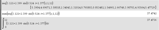
The total amount of rainfall (second line above) appears be R(1) + R(2) + R(3) + … +R(12) = 37.4742. This is very close to the amount calculated by integration.

The slight difference of 0.0006 is not a round off error.

Remember, behind every definite integral there is a Riemann sum!

Again, the units are the problem. Why does the sum of the monthly rates seem to give the total amount?  The reason is that the terms of the sequence above are actually the values of a right-side Riemann sum of the rate, R(t), over the interval [0,12] with 12 equal subdivisions of width 1 (month) each with the 1’s left out as 1’s often are. Therefore, their sum should come close to the total yearly rainfall, but it is really just an approximation of it.

The actual total for any month, n, is given by \displaystyle \int_{n-1}^{n}{r(t)}dt. For example the amount of rain that falls in June is given by \displaystyle \int_{5}^{6}{R(t)dt}=0.9890 inches.

Here is the sequence of the actual monthly rainfall values in inches, and their sum.

Ques 8 b

This agrees with the integral. Why? Because one of  the properties of integrals tell us that \displaystyle \sum\limits_{n=1}^{12}{\int_{n-1}^{n}{r(t)dt}}=\int_{0}^{12}{r(t)dt}.


Another instructive thing with this integral is this: The function R=3.121+2.399\sin \left( 0.524t+1.377 \right) is periodic with a period of  \frac{2\pi }{0.524}\approx 11.9908\approx 12. So the sine function takes on (almost) all its values in a year, as you would expect. Since the sine values all but cancel each other out

\displaystyle \int_{0}^{12}{3.121+2.399\sin \left( 0.524t+1.377 \right)dt}\approx \int_{0}^{12}{3.121dt=3.121\left( 12-0 \right)=37.452}. Close!

The total rainfall divided by 12 is \frac{37.452}{12}=3.121 this must be close to the average rainfall each month. The average rainfall is \displaystyle \frac{1}{12}\int_{0}^{12}{R\left( t \right)dt}=3.1228 inches. Close, again!


So, there you have it. Is this a good question or not? We considered all these concepts while working not just with an equation but with numbers from a poorly stated problem:

  • Reading and interpreting words.
  • Unit analysis
  • Integration by technology
  • Realizing that a pretty good approximation is not correct, due again to units.
  • A Riemann sum approximation in a real situation that comes very close to the value by integration
  • Using a property of a periodic function to greatly simplify an integral
  • Finding average value two ways

So, it turned out to be a sunny day in Seattle.seattle sun

.

Advertisement

Good Question 6: 2000 AB 4

2000 AB 4 Water tankAnother of my favorite questions from past AP exams is from 2000 question AB 4. If memory serves it is the first of what became known as an “In-out” question. An “In-out” question has two rates that are working in opposite ways, one filling a tank and the other draining it.

In subsequent years we saw a question with people entering and leaving an amusement park (2002 AB2/BC2), sand moving on and off a beach (2005 AB 2), another tank (2007 AB2), an oil leak being cleaned up (2008 AB 3), snow falling and being plowed (2010 AB 1), gravel being processed (2013 AB1/BC1), and most recently water again flowing in and out of a pipe (2015 AB1/BC1). The in-between years saw rates in one direction only but featured many of the same concepts.

The questions give rates and ask about how the quantity is changing. As such, they may be approached as differential equation initial value problems, but there is an easier way. This easier way is that a differential equation that gives the derivative as a function of a single variable, t, with an initial point \left( {{t}_{0}},y\left( {{t}_{0}} \right) \right) always has a solution of the form

y\left( t \right)=y\left( {{t}_{0}} \right)+\int_{{{t}_{0}}}^{t}{{y}'\left( x \right)dx}.

This is sometimes called the “accumulation equation.” The integral of a rate of change {y}'\left( t \right) gives the net amount of change over the interval of integration [{{t}_{0}},t]. When this is added to the initial amount the result is an expression that gives the amount at any time t.
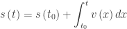
In a motion context, this same idea is that the position at any time t, is the initial position plus the displacement:

\displaystyle s\left( t \right)=s\left( {{t}_{0}} \right)+\int_{{{t}_{0}}}^{t}{v\left( x \right)dx} where v\left( t \right)={s}'\left( t \right)

The scoring standard gave both forms of the solution. The ease of the accumulation form over the differential equation solution was evident and subsequent standards only showed this one.

2000 AB 4

The question concerned a tank that initially contained 30 gallons of water. We are told that water is being pumped into the tank at a constant rate of 8 gallons per minute and the water is leaking out at the rate of \sqrt{t+1} gallons per minute.

Part a asked students to compute the amount of water that leaked out in the first three minutes. There were two solutions given. The second solves the problem as an initial value differential equation:

Let L(t) be the amount that leaks out in t minutes then

\displaystyle \frac{dL}{dt}=\sqrt{t+1}

L\left( t \right)=\frac{2}{3}{{\left( t+1 \right)}^{3/2}}+C

L\left( 0 \right)=\frac{2}{3}{{\left( 0+1 \right)}^{3/2}}+C=0 since nothing has leaked out yet, so C = -2/3
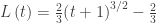
L\left( t \right)=\frac{2}{3}{{\left( t+1 \right)}^{3/2}}-\frac{2}{3}

L\left( 3 \right)=\frac{14}{3}

The first method, using the accumulation idea takes a single line:

\displaystyle L\left( 3 \right)=\int_{0}^{3}{\sqrt{t+1}dt}=\left. \frac{2}{3}{{\left( t+1 \right)}^{3/2}} \right|_{0}^{3}=\frac{2}{3}{{\left( 4 \right)}^{3/2}}-\frac{2}{3}{{\left( 1 \right)}^{3/2}}=\frac{14}{3}

I think you’ll agree this is easier and more direct.

Part b asked how much water was in the tank at t = 3 minutes.  We have 30 gallons to start plus 8(3) gallons pumped in and 14/3 gallons leaked out gives 30 + 24 – 14/3 = 148/3 gallons.

This part, worth only 1 point, was a sort of hint for the next part of the question.

Part c asked students to write an expression for the total number of gallons in the tank at time t.

Following part b the accumulation approach gives either

\displaystyle A\left( t \right)=30+8t-\int_{0}^{t}{\sqrt{x+1}dx}  or

\displaystyle A\left( t \right)=30+\int_{0}^{t}{\left( 8-\sqrt{x+1} \right)dx}.

The first form is not a simplification of the second, but rather the second form is treating the difference of the two rates, in minus out, as the rate to be integrated.

The differential equation approach is much longer and looks like this:

\displaystyle \frac{dA}{dt}=8-\sqrt{t+1}

A\left( t \right)=8t-\frac{2}{3}{{\left( t+1 \right)}^{3/2}}+C

A\left( 0 \right)=30=8(0)-\frac{2}{3}{{\left( 0+1 \right)}^{3/2}}+C, so C=\frac{92}{3}

A\left( t \right)=8t-\frac{2}{3}{{\left( t+1 \right)}^{3/2}}+\frac{92}{3}

Again, this is much longer. In recent years when asking student to write an expression such as this, the directions included a phrase such as “write an equation involving one or more integrals that gives ….” This pretty much leads students away from the longer differential equation initial value problem approach.

Part d required students to find the time when in the interval 0\le t\le 120 minutes the amount of water in the tank was a maximum and to justify their answer. The usual method is to find the derivative of the amount, A(t), set it equal to zero, and then solve for the time.

{A}'\left( t \right)=8-\sqrt{t+1}

Notice that this is the same regardless of which of the three forms of the expression for A(t) you start with. Thus, an excellent example of the Fundamental Theorem of Calculus used to find the derivative of a function defined by an integral. Or you could just start here without reference to the forms above: the overall rate in the rate in minus the rate out.

{A}'\left( t \right)=0 when t = 63

This is a maximum by the First Derivative Test since for 0 < t < 63 the derivative of A is positive and for 63 < t <120 the derivative of A is negative.

There is an additional idea on this part of the question in the Teaching Suggestions below.


I like this question because it is a nice real (as real as you can hope for on an exam) situation and for the way the students are led through the problem. I also like the way it can be used to compare the two methods of solution.  Then the way they both lead to the same derivative in part d is nice as well. I use this one a lot when working with teachers in workshops and summer institutes for these very reasons.

Teaching Suggestions

  • Certainly, have your students work through the problem using both methods. They need to learn how to solve an initial value problem (IVP) and this is good practice. Additionally, it may help them see how and when to use one method or the other.
  • Be sure the students understand why the three forms of A(t) in part c give the same derivative in part d. This makes an important connection with the Fundamental theorem of Calculus.
  • Like many good AP questions part d can be answered without reference to the other parts. The question starts with more water being pumped in than leaking out. This will continue until the rate at which the water leaks out overtakes the rate at which it is being pumped in. At that instant the rate “in” equals the rate “out” so you could start with 8=\sqrt{t+1}. After finding that t = 63, the answer may be justified by stating that before this time more water is being pumped in than is leaking out and after this time the rate at which water leaks out is greater than the rate at which it is pumped in, so the maximum must occur at t = 63.
  • And as always, consider the graph of the rates.

2000 AB 4

I used this question as the basis of a lesson in the current AP Calculus Curriculum Module entitled Integration, Problem Solving and Multiple Representations © 2013 by the College Board. The lesson gives a Socratic type approach to this question with a number of questions for each part intended to help the teacher not only work through this problem but to bring out related ideas and concepts that are not in the basic question. The module is currently available at AP sponsored workshops and AP Summer Institutes. Eventually, it will be posted at AP Central on the AB and BC Calculus Home Pages.

Good Question 5: 1998 AB2/BC2

Continuing my occasional series of some of my favorite teaching questions, today we look at the 1998 AP Calculus exam question 2. This question appeared on both the AB and BC exams. I use this problem to illustrate two very different questions that come up almost every time I lead a workshop or an AP Summer Institute. The first is if a limit is infinite, should you say “infinite” or “does not exist (DNE)”? The second is if the student solves the problems correctly, but by some other method, maybe even one not using the calculus, do they still earn full credit? In addition to discussing these two questions I’ll have a few suggestions for how to use this kind of question for teaching (maybe in other than a calculus class).

The question had the student examine the function f\left( x \right)=2x{{e}^{2x}} and, although it is easy enough to answer without, students were allowed to use their graphing calculator. A reasonable student probably looked at a graph of the function.
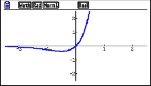
f\left( x \right)=2x{{e}^{2x}}

Part a: First the question asks the student to explore the end behavior of the function by finding two limits: \underset{x\to -\,\infty }{\mathop{\lim }}\,f\left( x \right) and \underset{x\to \infty }{\mathop{\lim }}\,f\left( x \right). The students should not depend on the graph here. As x\to -\infty , {{e}^{2x}}approaches zero and since the exponential function dominates the polynomial, \underset{x\to -\,\infty }{\mathop{\lim }}\,f\left( x \right)=0. In passing note that for x < 0 the function is negative and approaches zero from below. No work or explanation was required, but when teaching things like this be sure students know and can explain their answer without reference to their calculator graph.  For the second limit, since both factors increase without bound \underset{x\to \infty }{\mathop{\lim }}\,f\left( x \right)=\infty  If the student wrote \underset{x\to \infty }{\mathop{\lim }}\,f\left( x \right)=\text{DNE}, he received full credit.

Infinity is not a number, so there really is no limit in the second case; the limit DNE. But there are other ways a limit may not exist such as a jump discontinuity or an oscillating discontinuity.  DNE covers these as well as infinite limits. Saying a limit is infinite tells us more about the limit than DNE. It tells us that the function increases without bound; that eventually it becomes greater than any number.

Both answers are correct.

But we’re not done with this yet. We will come back to it before the question is done.

Part b: Students were asked to find and justify the minimum value of the function. Using the first derivative test, students proceeded by finding where the derivative is zero..

{f}'\left( x \right)=\left( 2x \right)\left( 2{{e}^{2x}} \right)+2{{e}^{2x}}=2{{e}^{2x}}\left( 2x+1 \right)=0

x=-\frac{1}{2}

f\left( -\tfrac{1}{2} \right)=2\left( -\tfrac{1}{2} \right){{e}^{2\left( -\tfrac{1}{2} \right)}}=-\frac{1}{e}\approx 0.368\text{ or }0.367

Justification: If x<-\tfrac{1}{2},\ {f}'\left( x \right)<0 and if x>-\tfrac{1}{2},\ {f}'\left( x \right)>0, therefore the absolute minimum is -\frac{1}{e} and occurs at x=-\frac{1}{2}.

All pretty straightforward

Part c: This part asked for the range of the function. Here the student must show that if he wrote DNE in part a, he knows that in fact the function grows without bound.

Putting together the answers from part a and part c, the range is f\left( x \right)\ge -\frac{1}{e}, which may also be written as \left[ -1/e,\infty\right). (The decimals could also be used here.)

Part d: asked students to consider functions given by y=bx{{e}^{bx}} where b was a non-zero number. The question required students to show that the absolute minimum value of all these functions was the same.

Most students did what was expected and preceded as in part b. The work is exactly the same as above except that all of the 2s become bs. The absolute minimum occurs at x=-\frac{1}{b} and y\left( -\tfrac{1}{b} \right)=-\frac{1}{e}.

BUT ….

Other students found a way completely without “calculus.” Can you find do that?

They realized that the given function as a horizontal expansion or compression, possibly including a reflection over the y-axis, of and therefore the range is the same for all these functions and so the minimum value must be the same. This received full credit. The rule of thumb is “don’t take off for good mathematics.”

Pretty cool!

The graphs of several cases are shown below

y=bx{{e}^{bx}}
b = -5 in blue, b = -1 in red, b = 2 in green, and b = 4 in magenta.

Teaching Suggestions

I can see using this in a pre-calculus class. The calculus (finding the minimum for b = 2 or in general) is straightforward. In a pre-calculus setting as an example of transformations it may be more useful. You could give students 6, or 8, or 10 examples with different values of b, both positive and negative.

  1. First ask students to investigate the end behavior by finding the limits as x approaches positive and negative infinity. The results will be similar. Have them write a summary considering two cases: b > 0 and b < 0.
  2. Graphing calculators have built-in operations that will find the x-coordinates or both coordinates of the minimum point of a function. Since we’re concerned with the transformation and not the calculus, let students use their graphing calculators to find the coordinates of the minimum point of each graph (as decimals). See if they can determine the x-coordinate in terms of b. They should also notice that y-coordinates will all be the same (about -0.367880).
  3. Finally, set the class to proving using their knowledge of transformation that the minimums are really all the same.

Good Question 3 1995 BC 5

A word before we look at one of my favorite AP exam questions, I put some of my presentations in a new page. Look under the “Resources” tab above, and you will see a new page named “Presentations.” There are PowerPoint slides and the accompanying handouts from some talks I’ve given in the last few years. I also use them in my workshops and AP Summer Institutes.

This continue a discussion of some of my favorite question and how to use them in class.You can find the others by entering “Good Question” in the search box on the right.

Today we look at one of my favorite AP exam questions. This one is from the 1995 BC exam; the question is also suitable for AB students. Even though it is 20 years old, it is still a good question.  1995 was the first year that graphing calculators were required on the AP Calculus exams.They were allowed, but not required for all 6 questions.

1995 BC 5

The question showed the three figures below and identified figure 1 as the graph of f\left( x \right)={{x}^{2}}  
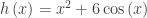
and figure 2 as the graph of g\left( x \right)=\cos \left( x \right).  The question then allowed as how one might think of the graph is figure 3 as the graph of h\left( x \right)={{x}^{2}}+\cos \left( x \right), the sum of these two functions. Not that unreasonable an assumption, but apparently not correct.

1995 BC 5

Part a: The students first were asked to sketch the graph of h\left( x \right) 
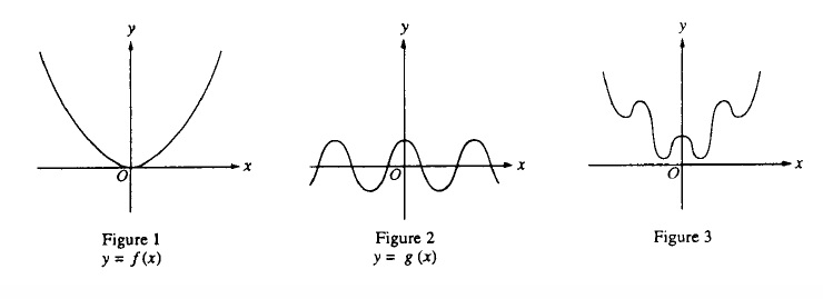
in a window with [–6, 6] x [–6, 40] (given this way). A box with axes was printed in the answer booklet.  This was a calculator required question and the result on a graphing calculator looks like this:


1995 BC 5

y={{x}^{2}}+\cos \left( x \right).
The window is [-6,6] x [-6, 40]

Students were expected to copy this onto the answer page. Note that the graph exits the screen below the top corners and it does not go through the origin. Both these features had to be obvious on the student’s paper to earn credit.

Part b: The second part of the question instructed students to use the second derivative of h\left( x \right) to explain why the graph does not look like figure 3.

\displaystyle \frac{dy}{dx}=2x-\sin \left( x \right)

\displaystyle \frac{{{d}^{2}}y}{d{{x}^{2}}}=2-\cos \left( x \right)

Students then had to observe that the second derivative was always positive (actually it is always greater than or equal to 1) and therefore the graph is concave up everywhere. Therefore, it cannot look like figure 3.

Part c: The last part of the question required students to prove (yes, “prove”) that the graph of y={{x}^{2}}+\cos \left( kx \right) 
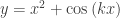
either had no points of inflection or infinitely many points of inflection, depending on the value of the constant k.
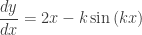
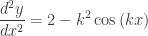
Successful student first calculated the second derivative:

\displaystyle \frac{dy}{dx}=2x-k\sin \left( kx \right)

\displaystyle \frac{{{d}^{2}}y}{d{{x}^{2}}}=2-{{k}^{2}}\cos \left( kx \right)

Then considering the sign of the second derivative, if {{k}^{2}}\le 2, \frac{{{d}^{2}}y}{d{{x}^{2}}}\ge 0 and there are no inflection points (the graph is always concave up). But, if {{k}^{2}}>2, then since y” is periodic and changes sign, it does so infinitely many times and there are then infinitely many inflection points. See the figure below.

k = 8

k = 8


Using this question as a class exercise

Notice how the question leads the student in the right direction. If they go along with the problem they are going in the right direction. In class, I would be inclined to make them work for it.

  1. First, I would ask the class if figure 3 is the correct graph of h\left( x \right)={{x}^{2}}+\cos \left( x \right). I would let them, individually, in groups, or as a class suggest and defend an answer. I would not even suggest, but certainly not mind, if they used a graphing calculator.
  2. Once they determined the correct answer, I would ask them to justify (or prove) their conjecture. Again, no hints; let the class struggle until they got it. I may give them a hint along the lines of what does figure 3 have or do that the correct graph does not. (Answer: figure 3 changes concavity). Sooner or later someone should decide to check out the second derivative.
  3. Then I’d ask what could be the equation for a graph that does look like figure 3. You could give hints along the line of changing the coefficients of the terms of the second derivative. There are several ways to do this and all are worth considering.
    1. Changing the coefficient of the x2 term (to a proper fraction, say, 0.02) will do the trick. If that’s what they come up with fine – it’s correct.
    2. If you want to be picky, this causes the graph to go negative and figure 3 does not do that, but I ‘d let that go and ask if changing the coefficient of the cosine term in the second derivative can be done and if so how do you do that.
    3. This may be done by simply putting a number in front of the cosine term of the original function, say h\left( x \right)={{x}^{2}}+6\cos \left( x \right)
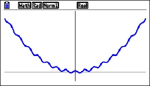
, but the results really do not look like figure 3,
    4. If necessary, give them the hint y={{x}^{2}}+\cos \left( kx \right)

1995 was the first year graphing calculators were required on the AP Calculus exams. They were allowed for all questions, but most questions had no place to use them. The parametric equation question on the same test, 1995 BC 1, was also a good question that made use of the graphing capability of calculators to investigate the relative motion of two particles in the plane.   The AB Exam in 1995 only required students to copy one graph from their calculator.

Both BC questions were generally well received at the reading. I know I liked them. I was looking forward to more of the same in coming years.

I was disappointed.

There was an attempt the following year (1997 AB4/BC4), but since then nothing investigating families of functions (i.e.  like these with a parameter that affects the shape of the graph) or anything similar has appeared on the exams. I can understand not wanting to award a lot of points for just copying the graph from your calculator onto the paper, but in a case like this where the graph leads to a rich investigation of a counterintuitive situation I could get over my reluctance.

But that’s just me.