I guess the obvious answer is so you will have something to use your new knowledge of the definite integral on. This unit is a collection of the first applications. There are many more.
The whole idea is based on the fact that a definite integral is a sum. Thus, they can be used to add things. Complicated shapes can be divided into simple shapes, like rectangles, and their areas can be added.
Here are the first uses.
AVERAGE VALUE OF A FUNCTION ON AN INTERVAL
You know that to average two numbers you add them and divide the total by two. To average a larger set of numbers you add them and divide the sum by the number of numbers. Now you will learn how to average the infinite number of y-values of a function over an interval. To do it you use a definite integral.
HINT: Average value of a function, average rate of change of a function, and the mean value theorem all sound kind of the same. Furthermore, the formulas all look kind of the same. Don’t mix them up. Use their full name, not just “average,” and use the right one.
There is an interesting result found some years ago by a tenth-grade student who took AB Calculus in eighth grade and BC in ninth. He proved that Most Triangles Are Obtuse! using the average value integral.
LINEAR MOTION
This application extends your previous work on objects moving on a line. By adding, with a definite integral, you will be able to determine how far the object moves in a given time. Knowing that and where the object starts, you will be able to find its current position. BC students will also learn how to find the length of a curve in the plane.
THE AREA BETWEEN TWO CURVES
This application extends what you know about finding the area between a curve and the x-axis to finding the area between two curves.
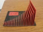
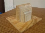
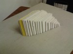
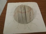
VOLUME OF A SOLID FIGURE WITH A REGULAR CROSS-SECTION
Some solid objects, when sliced in the right way, have regular cross-section. That means, the cut surface is a square, a rectangle, a right triangle, a semi-circle and so on. Think of cutting a piece of butter from a stick of butter – each piece is a square with a little thickness, like a very small pizza box. By using an integral to add their volumes you can find the volume of the original figure. .
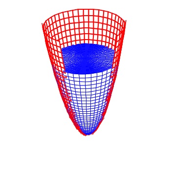
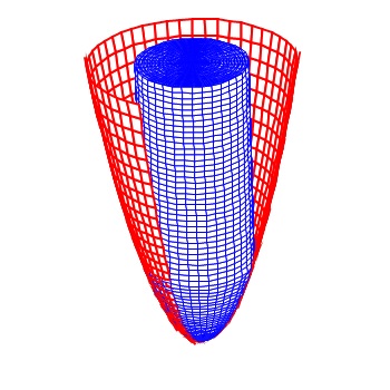
VOLUME OF A SOLID OF REVOLUTION – DISK METHOD
A region in the plane is revolved aroud a line resulting in a solid figure. Finding its volume is just a special case of a solid with regular cross section where the cross section is a circle. Each little piece is a disk. By adding their volumes with an integral you can calculate the volume.
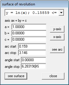
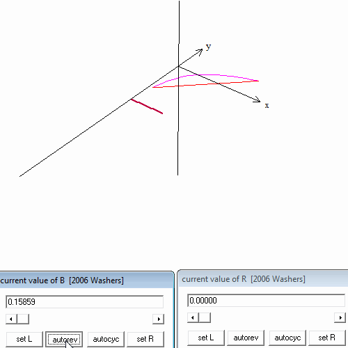
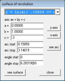
VOLUME OF A SOLID OF REVOLUTION – WASHER METHOD
Some solids of revolution have holes through them. These are formed by revolving a plane figure (usually the region between two curves) around an edge or a line outside the figure. The line is often the x– or y-axis. There is a formula for doing this, but understanding what you are doing – doing two disk problems – will help you with doing this. (See Subtract the Hole from the Whole.)
One last hint: You will want to know what the solid figure looks like. In addition to the illustrations in your textbook, there are various places online where you can find pictures of the figures. You can build models of them. There is an excellent iPad app called A Little Calculus that does a good job of illustrating and animating solid figures (and lots of other calculus stuff).
Course and Exam Description Unit 8


 and the line
  both for
  .
.

 , so
, so 
 and
and 


 and
and  from x = 1 to x = 5.
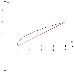
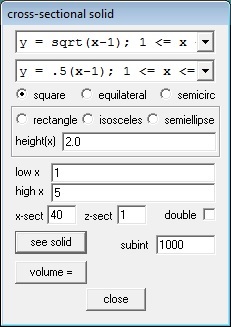
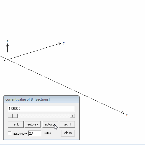
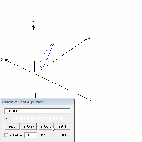
 Now let’s get fancy. Close the 3D window and return to the cross-section box shown above. Change the “high x” to 5@B (you may use any almost letter except x, y, or z). Then click “see solid.” Next, in the 3D Window click Anim > Individual > B. This will give you a slider. Slide the slider from 1 to 5 and you will see the solid grow and see the square cross-sections. (The video uses the “autocyc” button – use S to slow the animation, F to speed it up and Q to quit.)