Visualizing Solid Figures 2

Posted on November 16, 2014 by Lin McMullin

You have probably caught on by now that Winplot is my favorite computer graphing program. In addition to being great at drawing quick graphs, it is able to produce and rotate 3D images of, among other things, solids of rotation, and solids with regular cross-sections. In this post I will discuss how to do solids of regular cross-section and solids of rotation. In my next posts I’ll show you how to see the disks, washers, and shells.

Winplot is a free program. Click here for Winplot for PC and here for Winplot for Macs. (May 11, 2017 Note: Winplot is no longer available from its original home. The link for PCs above connect to another site where the program can be downloaded. For Macs use the PC link, but use the Winplot for Macs link for instructions and another program you will need.You can also Google Winplot and find other sites that have the program as well as many, many instructional videos.)

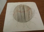
Solids with regular cross-sections

Consider the region bound by the graphs of 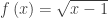$f\left( x \right)=\sqrt{x-1}$ and $g\left( x \right)=\tfrac{1}{2}\left( x-1 \right)$ from x = 1 to x = 5.

Begin by opening a Winplot 2D graphing window, graphing the curves, and adjusting the window to a good scale. Use the box where the equations are entered (Equa > 1.Explicit) check “lock interval,” and enter the “low x” and “high x” values (1 and 5 respectively) to stop the graphs where they intersect. Click “ok” to see the graphs.

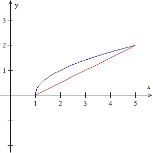
On the navigation bar, click on “Two” and then “Sections.” You should see a window like this:

The top two drop-down boxes at the top allow you to choose which curves to work with, and since we have only two they should already be selected. Then click on the cross-section shape you want – square, equilateral triangle, or semicircle. The box below that allows other shapes where the height may be set (the height(x) may be a number or a function of x). Set the “low x” and “high x” to the left and right sides of the region. Then click “see solid” and you will see the solid in a new window.

Click on the new 3D window and then type Ctrl+A to show the axes. Rotate the image by using the 4 arrow keys, and zoom in and out with the Page Up and Page Down keys.

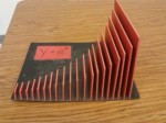
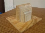
Now let’s get fancy. Close the 3D window and return to the cross-section box shown above. Change the “high x” to 5@B (you may use any almost letter except x, y, or z). Then click “see solid.” Next, in the 3D Window click Anim > Individual > B. This will give you a slider. Slide the slider from 1 to 5 and you will see the solid grow and see the square cross-sections. (The video uses the “autocyc” button – use S to slow the animation, F to speed it up and Q to quit.)

Use File > Save As… to save the image. It will save with the extension .wp3 and you will lose the original 2D graphs. The animation buttons will still work when you open it again.

Solids of Revolution.

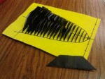
Solids of rotation are done in a similar way. We will revolve the same curves around the horizontal line y = –1. Enter the curves as above and click on One > Revolve Surface. Curves are revolved one at a time, so choose the first curve from the drop-down box. Choose the axis the figure is to be rotated around by entering the values for a, b, and c in ax + by = c, or clicking on one of the axis buttons. For the “arc start” and “arc stop” values use the left and right ends of the region. The “angle start” and “angle stop” values are the default, 0 and 2pi (entered as “2pi”). Again we have made this last value 2pi@A so that we can animate the graph.

Click “see surface” to see the revolved surface. As before, use the 4 arrow keys and the Page Up and Page Down keys to adjust the image, and Ctrl+A to show the axes.

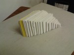
Surfaces are revolved one at a time so return to the “surface of revolution” window and use the drop-down box to choose the next curve. Leave all the other values the same. Clicking “see surface” will graph the second curve with the first and show the solid figure. Note that the surfaces are graphed in the same color as the original 2D graphs.

Use the slider or autorev or autocyc buttons to watch the curves revolve. (Remember to type “F” to speed up the motion. “S” to slow it down, and “Q” to quit.)

The next posts will show how to see the disks, washers, and shells, and animate them along with the surfaces.

Visualizing Solid Figures 1

Posted on November 13, 2014 by Lin McMullin

The shape of various solids of rotation and solids with regular cross-sections of which beginning calculus students are required to find the volume are often difficult to visualize. This post and the next two will discuss some of the ways you can help your students become familiar with these shapes. Teachers often use these as projects for students to get some hands-on familiarity with the figures. In fact, it is one of the few places where a useful project can be assigned.

Actually, rotate a region:

Begin by drawing the region to be revolved (from the curve to the line of rotation) on paper and cut it out. Tape the region along the line to a pencil, pen, or dowel. Roll the dowel back and forth between your hands or, as shown in the video below, with a small electric drill or screwdriver. You can get a rough idea of the shape.

Go to a wedding:

Decorations for weddings and other festive events are made from paper and fold flat. When opened you get a solid of rotation.

Measure a volume:

Take a solid fruit (like a banana), or a vegetable (like a cucumber, or carrot) and find its volume by cutting it into “coin” shaped pieces. Multiply the thickness by the area of the circular ends of each piece and then add them to find the volume.

For more of a challenge use a loaf of sliced bread (here you will need a way to calculate the area of the non-circular ends – inscribed rectangles perhaps). You could also approximate the volume of a tree trunk by measuring the circumference at regular distances along the trunk.

Build a model:

This method can be used for solids or rotation and is especially good for solids with regular cross-sections. It is also a good project for a student or group of students.

Carefully graph the region using a somewhat larger than normal scale.
Draw lines at 1/8 to ¼ inch intervals across the region perpendicular to the appropriate axis.
Carefully measure or calculate the length of each of these lines. Use this for the appropriate dimension for the question. For example, this may be the side of the square cross-section, or the diameter of a semi-circular section.
Use the dimension to draw a series of squares, semi-circles, or whatever from cardboard, plywood, or foam board.
Cut these out and assemble them on the original region you graphed to approximate the solid figure. Tape or glue them in place.
Extra: Calculate the area of each piece and multiply it by the thickness (or the distance between pieces) and see how closely this comes to the calculated volume.

: Square cross-sections from scrap wood.

: Square cross-sections on a circular base made from scrap plywood.

: Trapezoidal sections on parabolic base made from 5.25 inch floppy disks.

: Square cross-sections on base between a parabola and a line made with foam board.

: Semi-circular cross-sections on a circular base made from foam board.

These pictures are of models made by students of Mrs. Dixie Ross at Pflugerville (Texas) High School. Students received more points if they recycled materials.Thank you Dixie!

Improper Integrals and Proper Areas

Posted on January 25, 2014 by Lin McMullin

A few years ago, on the old AP Calculus discussion group a teacher asked a question about this improper integral:

$\displaystyle \int_{0}^{\infty }{\frac{1}{1+{{x}^{2}}}dx}=\underset{b\to \infty }{\mathop{\lim }}\,\int_{0}^{b}{\frac{1}{1+{{x}^{2}}}dx}$

$=\underset{b\to \infty }{\mathop{\lim }}\,\left. \left( {{\tan }^{-1}}\left( x \right) \right) \right|_{0}^{b}$

$=\underset{b\to \infty }{\mathop{\lim }}\,\left( {{\tan }^{-1}}\left( b \right)-{{\tan }^{-1}}\left( 0 \right) \right)=\frac{\pi }{2}$

His (quite perceptive) student pointed out that the range of the inverse tangent function is arbitrarily restricted to the open interval $\left( -\tfrac{\pi }{2},\tfrac{\pi }{2} \right)$ . The student asked if some other range would affect the answer to this problem. The short answer is no, the result is the same. For example, if range were restricted to say $\left( \tfrac{5\pi }{2},\tfrac{7\pi }{2} \right)$ , then in the computation above:

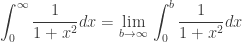
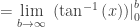
$\underset{b\to \infty }{\mathop{\lim }}\,\left( {{\tan }^{-1}}\left( b \right)-{{\tan }^{-1}}\left( 0 \right) \right)=\tfrac{7\pi }{2}-3\pi =\tfrac{\pi }{2}$

The value is the same. While that is pretty straightforward, there are other things going on here which may be enlightening. The original indefinite integral represents the area in the first quadrant between the graph of $y=\frac{1}{1+{{x}^{2}}}$ and the x-axis. Let’s consider the function that gives the area between the y-axis and the vertical line at various values of x.

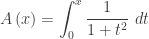
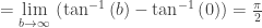
$A \displaystyle\left( x \right)=\int_{0}^{x}{\frac{1}{1+{{t}^{2}}}}\ dt$

Pretending for the moment that we don’t know the antiderivative, we can use a calculator to graph the area function. Of course, we recognize this as the inverse tangent function, but what is more interesting is that whatever this function is, it seems to have a horizontal asymptote at $y=\tfrac{\pi }{2}$ . The area is approaching a finite limit as x increases without bound. The unbounded region has a finite area. The connection with improper integrals is obvious.

$\displaystyle \underset{b\to \infty }{\mathop{\lim }}\,A\left( b \right)=\underset{b\to \infty }{\mathop{\lim }}\,\int_{0}^{b}{\frac{1}{1+{{x}^{2}}}dx=}\int_{0}^{\infty }{\frac{1}{1+{{x}^{2}}}dx}$

Also, the improper integral is defined as the limit of the area function. This may give some insight as to why improper integrals are defined as they are.

Stamp Out Slope-intercept Form!

Posted on January 30, 2013 by Lin McMullin

Accumulation 5: Lines

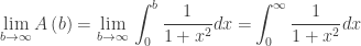
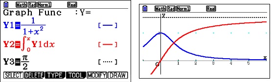
If you have a function y(x), that has a constant derivative, m, and contains the point $\left( {{x}_{0}},{{y}_{0}} \right)$ then, using the accumulation idea I’ve been discussing in my last few posts, its equation is

$\displaystyle y={{y}_{0}}+\int_{{{x}_{0}}}^{x}{m\,dt}$

$\displaystyle y={{y}_{0}}+\left. mt \right|_{{{x}_{0}}}^{x}$

$\displaystyle y={{y}_{0}}+m\left( x-{{x}_{0}} \right)$

This is why I need your help!

I want to ban all use of the slope-intercept form, y = mx + b, as a method for writing the equation of a line!

The reason is that using the point-slope form to write the equation of a line is much more efficient and quicker. Given a point $\left( {{x}_{0}},{{y}_{0}} \right)$ and the slope, m, it is much easier to substitute into $y={{y}_{0}}+m\left( x-{{x}_{0}} \right)$ at which point you are done; you have an equation of the line.

Algebra 1 books, for some reason that is beyond my understanding, insist using the slope-intercept method. You begin by substituting the slope into $y=mx+b$ and then substituting the coordinates of the point into the resulting equation, and then solving for b, and then writing the equation all over again, this time with only m and b substituted. It’s an algorithm. Okay, it’s short and easy enough to do, but why bother when you can have the equation in one step?

Where else do you learn the special case (slope-intercept) before, long before, you learn the general case (point-slope)?

Even if you are given the slope and y-intercept, you can write $y=b+m\left( x-0 \right)$ .

If for some reason you need the equation in slope-intercept form, you can always “simplify” the point-slope form.

But don’t you need slope-intercept to graph? No, you don’t. Given the point-slope form you can easily identify a point on the line, $\left( {{x}_{0}},{{y}_{0}} \right)$ , start there and use the slope to move to another point. That is the same thing you do using the slope-intercept form except you don’t have to keep reminding your kids that the y-intercept, b, is really the point (0, b) and that’s where you start. Then there is the little problem of what do you do if zero is not in the domain of your problem.

Help me. Please talk to your colleagues who teach pre-algebra, Algebra 1, Geometry, Algebra 2 and pre-calculus. Help them get the kids off on the right foot.

Whenever I mention this to AP Calculus teachers they all agree with me. Whenever you grade the AP Calculus exams you see kids starting with y = mx + b and making algebra mistakes finding b.

AP Accumulation Questions

Posted on January 23, 2013 by Lin McMullin

Accumulation 2: AP Exam Rate/Accumulation Questions

I assume that a number of my readers are AP Calculus teachers. In following up my last post on accumulation, today I’m going to discuss a very common type of AP Calculus exam question, the rate question which is loaded with accumulation ideas. The three posts following this one will show how accumulation can help with graphing problems.

If you do not have them, these two links will take you to them. Click on the question number for links to the question and scoring standard.

2000 AB 4: In this questions water was being pumped into a tank at the constant rate of 8 gallons per minute and leaking out at the rate of $\sqrt{t+1}$ gallons per minute. At time t = 0 we are told there are 30 gallons of water in the tank. (Many AP exams problems have two rates acting at the same time, one increasing the amount and the other decreasing it.)

The first part of the question asked for the amount of water that leaked out of the tank in the first 3 minutes. This is like the situation discussed in the last post: If you need an amount, look around for a rate to integrate. The answer is $\displaystyle\int_{0}^{3}{\sqrt{t+1}dt}=\tfrac{14}{3}\text{ gallons}\text{.}$

The next part asked for the amount of water in the tank after t minutes. So, we start with 30 gallons and add the amount put in which is 8 gallons per minute for 3 minutes of 24 gallons. Of course, we could also get this by integrating $\displaystyle \int_{0}^{3}{8dt}=24$ . Then we subtract the amount that leaked out from the first part. The amount is 30 + 24 – 14/3 gallons. This was to help students with the next part.

The third part asked for an expression for A(t), the amount of water at any time t. So following on the second part we have either $\displaystyle A\left( t \right)=30+8t-\int_{0}^{x}{\sqrt{t+1}dt}$ or $\displaystyle A\left( t \right)=30+\int_{0}^{x}{8-\sqrt{t+1}\,dt}$ . Either form, especially the latter, is the form of an accumulation function: the initial amount plus the integral of the rate of change. It was not required to actually do the integration, but if someone did then $\displaystyle A\left( t \right)=8t-\tfrac{2}{3}{{\left( t+1 \right)}^{3/2}}+\tfrac{92}{3}$

The last part asked when the maximum amount of water was in the tank. As in any extreme value problem you can find this by differentiating any of the expressions for the amount found in the third part: ${A}'\left( t \right)=8-\sqrt{t+1}$ by the FTC. (This could also be found by simply subtracting the two rates.) This will change from positive to negative when t = 63; this is when the maximum amount of water is in the tank. Notice that this is when the amount leaking out becomes greater than the amount being pumped into the tank; the total change becomes negative.

2009 AB 3: This question had a different twist or two on the accumulation idea. This proved rather difficult for the majority of the students (The mean score was 1.92 out of a possible 9 points.) The problem said that the Mighty Cable Company sold their cable for $120 per meter. The cost of producing the cable was given as $6\sqrt{x}$ dollars per meter. (Notice that these are rates as evidenced by their units $/m; the word “rate” was not used. It is important that students recognize when something is a rate.) The stem also defined profit as the difference between the amount of money received for the cable and the cost of producing the cable.

The first part of the question asked for the profit on 25 meters of cable. The amount the company receives is 25 meters times $120 dollars per meter (an amount so we could integrate the rate here, but that’s overkill). The amount the 25 meters costs to produce is (remember if you need an amount, integrate the rate): $\displaystyle \int_{0}^{25}{6\sqrt{x}\,dx}$ , so the $\displaystyle \text{Profit }=120\cdot 25-\int_{0}^{25}{6\sqrt{x}\,dx}=\$2,500$

The third part built on the first part by asking for the profit earned for a cable k meters long: $\displaystyle \text{Profit =}120k-\int_{0}^{k}{6\sqrt{x}\,dx}$ or $\displaystyle P(x)=\int_{0}^{k}{120-6\sqrt{x}\,dx}$ . There is your accumulation function. The initial value is $0.

The second part was the most interesting. In it students were asked to explain the meaning of $\displaystyle \int_{25}^{30}{6\sqrt{x}\,dx}$ in the context of the problem. One way to see what this represents is to think about the FTC. The integral of the rate in dollars per meter is the cost per meter. If we call the cost C, then $\displaystyle \int_{25}^{30}{6\sqrt{x}\,dx}=C\left( 30 \right)-C\left( 25 \right)$ . Now students did not need to do a computation here; they just have to read what the symbols mean. $C\left( 30 \right)-C\left( 25 \right)$ is the difference between the cost of manufacturing a 25-meter cable and a 30-meter table. When you integrate a rate, you get the net amount.

As in the previous question the fourth part asked for the maximum profit. This was found by differentiating the profit expression from the third part by the FTC, ${P}'\left( x \right)=120-6\sqrt{x}$ and finding when the derivative changed from positive to negative, at x = 400 meters and substituting this into the profit equation.

Area Between Curves

Posted on January 7, 2013 by Lin McMullin

Applications of Integration 1 – Area Between Curves

The first thing to keep in mind when teaching the applications of integration is Riemann sums. The thing is that when you set up and solve the majority of application problems you cannot help but develop a formula for the situation. Students think formulas are handy and go about memorizing them badly. By which I mean they forget or never learn where the various things in the formula come from. A slight change in the situation and they are lost. Behind every definite integral stands a Riemann sum; each application should be approached through its Riemann sum. If students understand that, they will make fewer mistakes with the “formula.”

As I suggested in a previous post, I believe all area problems should be treated as the area between two curves. If you build the Riemann sum rectangle between the graph and the axis and calculate its vertical side as the upper function minus the lower (or right minus left if you use horizontal rectangles) you will always get the correct integral for the area. If the upper curve is the x-axis, then the vertical sides of the Riemann sums are (0 – f(x)) and you get a positive area as you should.

If both your curves are above the x-axis, then it is tempting to explain what you are doing as subtracting the area between the lower curve and the x-axis from the area between the upper curve and the x-axis. And this is not wrong. It just does not work very smoothly when one, both or parts of either are below the x-axis. Then you go into all kinds of contortions explaining things in terms of positive and negative areas. Why go there?

Regardless of where the two curves are relative to the x-axis, the vertical distance between them is the upper value minus the lower, f(x) – g(x). It does not matter if one or both functions are negative on all or part of the interval, the difference is positive and the area between them is

$\displaystyle \underset{n\to \infty }{\mathop{\lim }}\,\sum\limits_{i=1}^{n}{\left( f\left( {{x}_{i}} \right)-g\left( {{x}_{i}} \right) \right)\Delta {{x}_{i}}}=\int_{a}^{b}{f\left( x \right)-g\left( x \right)dx}$ .

Furthermore, this Riemann sum rectangle is used in other applications. It is the one rotated in both the washer and shell method of finding volumes. So in area and all applications be sure your students don’t just memorize formulas, but keep their eyes on the rectangle and the Riemann sum.

Finally, if the graphs cross in the interval so that the upper and lower curves change place, you may (1) either break the problem into several pieces so that your integrands are always of the form upper minus lower, or (2) if you intend to do the computation using technology, set up the integral as

$\displaystyle \int_{a}^{b}{\left| f\left( x \right)-g\left( x \right) \right|dx}$ .

Teaching Calculus

The pleasure lies not in discovering the truth, but in searching for it.

Tag Archives: Jan.

Visualizing Solid Figures 2

Visualizing Solid Figures 1

Improper Integrals and Proper Areas

Stamp Out Slope-intercept Form!

AP Accumulation Questions

Area Between Curves

Share this:

Like this:

Share this:

Like this:

Share this:

Like this:

Share this:

Like this:

Share this:

Like this:

Share this:

Like this: