
AP Questions Type 2: Linear Motion
We continue the discussion of the various type questions on the AP Calculus Exams with linear motion questions.
“A particle (or car, person, or bicycle) moves on a number line ….”
These questions may give the position equation, the velocity equation (most often), or the acceleration equation of something that is moving on the x– or y-axis as a function of time, along with an initial condition. The questions ask for information about motion of the particle: its direction, when it changes direction, its maximum position in one direction (farthest left or right), its speed, etc.
The particle may be a “particle,” a person, car, a rocket, etc. Particles don’t really move in this way, so the equation or graph should be considered to be a model. The question is a versatile way to test a variety of calculus concepts since the position, velocity, or acceleration may be given as an equation, a graph, or a table; be sure to use examples of all three forms during the review.
Many of the concepts related to motion problems are the same as those related to function and graph analysis (Type 3). Stress the similarities and show students how the same concepts go by different names. For example, finding when a particle is “farthest right” is the same as finding the when a function reaches its “absolute maximum value.” See my post for Motion Problems: Same Thing, Different Context for a list of these corresponding terms. There is usually one free-response question and three or more multiple-choice questions on this topic.
The position, s(t), is a function of time. The relationships are:
- The velocity is the derivative of the position,
. Velocity is has direction (indicated by its sign) and magnitude. Technically, velocity is a vector; the term “vector” will not appear on the AB exam.
- Speed is the absolute value of velocity; it is a number, not a vector. See my post for Speed.
- Acceleration is the derivative of velocity and the second derivative of position,
. It, too, has direction and magnitude and is a vector.
- Velocity is the antiderivative of the acceleration.
- Position is the antiderivative of velocity.
What students should be able to do:
- Understand and use the relationships above.
- Distinguish between position at some time and the total distance traveled during the time period.
- The total distance traveled is the definite integral of the speed (absolute value of velocity)
.
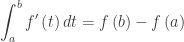
- Be sure your students understand the term displacement; it is the net distance traveled or distance between the initial position and the final position. Displacement, is the definite integral of the velocity (rate of change):
.
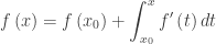
- The final position is the initial position plus the displacement (definite integral of the rate of change from x= a to x = t):
Notice that this is an accumulation function equation (Type 1).
- Initial value differential equation problems: given the velocity or acceleration with initial condition(s) find the position or velocity. These are easily handled with the accumulation equation in the bullet above, but may also be handled as an initial value problem.
- Find the speed at a given time. The speed is the absolute value of the velocity.
- Find average speed, velocity, or acceleration
- Determine if the speed is increasing or decreasing.
- If at some time, the velocity and acceleration have the same sign then the speed is increasing.If they have different signs the speed is decreasing.
- If the velocity graph is moving away from (towards) the t-axis the speed is increasing (decreasing). See the post on Speed.
- There is also a worksheet on speed here
- The analytic approach to speed: A Note on Speed
- Use a difference quotient to approximate the derivative (velocity or acceleration) from a table. Be sure the work shows a quotient.
- Riemann sum approximations.
- Units of measure.
- Interpret meaning of a derivative or a definite integral in context of the problem
Shorter questions on this concept appear in the multiple-choice sections. As always, look over as many questions of this kind from past exams as you can find.
This may be an AB or BC question. The BC topic of motion in a plane, (Type 8: parametric equations and vectors) will be discussed in a later post.
The Linear Motion problem may cover topics primarily from primarily from Unit 4, and also from Unit 3, Unit 5, Unit 6, and Unit 8 (for BC) of the 2019 CED.
Free-response examples:
- Equation stem 2017 AB 5,
- Graph stem: 2009 AB1/BC1,
- Table stem 2019 AB2
Multiple-choice examples from non-secure exams:
- 2012 AB 6, 16, 28, 79, 83, 89
- 2012 BC 2, 89
 ,
, is the initial time, and
  is the initial amount. Since this is one of the main interpretations of the definite integral the concept may come up in a variety of situations.
 is the initial time, and
  . Discuss the graph of the relation giving reasons for your conclusions. Include a brief mention of any unproductive paths you followed and what you learned from them.
 .
. and
and  . What does this say about the graph?
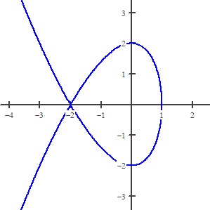
 . Values greater than 1 will make the left side of the equation greater than 4 regardless of the value of y. The range of the relation is all real numbers.
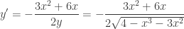 by implicit differentiation or by differentiating the equation for the top half.
 does not exist at x = 1 specifically,
  . Therefore, the line x = 1 is a vertical tangent. By symmetry for the lower part of the graph
  . And x = 1 is its vertical asymptote as well. The slope of the original relation changes from positive to negative at x = 1 by going not through zero but from
  to
to  .
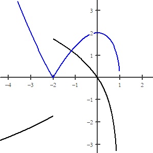
. when x = 0 and when x = –2. At (0, 2) the derivative changes from positive to negative; this is a local maximum point by the first derivative test. The lower half has a local minimum point at (0, –2) by symmetry.
 .
.

 and
and 
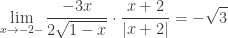
 and on the right approaches
  .
. and
and  . (Other forms may be included, but only these two are tested on the AP exams.)


 , so, substituting
  we have


 – Fermat unknowingly is using the derivative! After which he set it equal to 0 and solved to find the
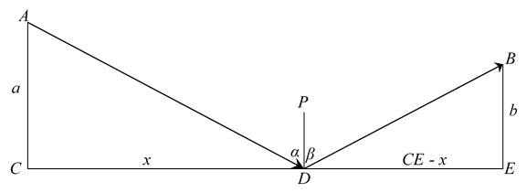
 and
and  are all perpendicular to
  the total distance is AD + DB. Therefore:
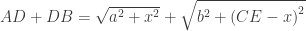


 and
and
 QED.
QED.
 with a > b > 0. Solving for y there are two equations, the second one is for the upper half that we will use below. The other for the lower half.
 and
and  .
. to avoid working with an undefined slope. The focus is at
  .
.