
Unit 5 covers the application of derivatives to the analysis of functions and graphs. Reasoning and justification of results are also important themes in this unit. (CED – 2019 p. 92 – 107). These topics account for about 15 – 18% of questions on the AB exam and 8 – 11% of the BC questions.
You may want to consider teaching Unit 4 after Unit 5. Notes on Unit 4 are here.
Reasoning and writing justification of results are mentioned and stressed in the introduction to the topic (p. 93) and for most of the individual topics. See Learning Objective FUN-A.4 “Justify conclusions about the behavior of a function based on the behavior of its derivatives,” and likewise in FUN-1.C for the Extreme value theorem, and FUN-4.E for implicitly defined functions. Be sure to include writing justifications as you go through this topic. Use past free-response questions as exercises and also as guide as to what constitutes a good justification. Links in the margins of the CED are also helpful and give hints on writing justifications and what is required to earn credit. See the presentation Writing on the AP Calculus Exams and its handout
Topics 5.1
Topic 5.1 Using the Mean Value Theorem While not specifically named in the CED, Rolle’s Theorem is a lemma for the Mean Value Theorem (MVT). The MVT states that for a function that is continuous on the closed interval and differentiable over the corresponding open interval, there is at least one place in the open interval where the average rate of change equals the instantaneous rate of change (derivative). This is a very important existence theorem that is used to prove other important ideas in calculus. Students often confuse the average rate of change, the mean value, and the average value of a function – See What’s a Mean Old Average Anyway?
Topics 5.2 – 5.9
Topic 5.2 Extreme Value Theorem, Global Verses Local Extrema, and Critical Points An existence theorem for continuous functions on closed intervals
Topic 5.3 Determining Intervals on Which a Function is Increasing or Decreasing Using the first derivative to determine where a function is increasing and decreasing.
Topic 5.4 Using the First Derivative Test to Determine Relative (Local) Extrema Using the first derivative to determine local extreme values of a function
Topic 5.5 Using the Candidates’ Test to Determine Absolute (Global) Extrema The Candidates’ test can be used to find all extreme values of a function on a closed interval
Topic 5.6 Determining Concavity of Functions on Their Domains FUN-4.A.4 defines (at least for AP Calculus) When a function is concave up and down based on the behavior of the first derivative. (Some textbooks may use different equivalent definitions.) Points of inflection are also included under this topic.
Topic 5.7 Using the Second Derivative Test to Determine Extrema Using the Second Derivative Test to determine if a critical point is a maximum or minimum point. If a continuous function has only one critical point on an interval then it is the absolute (global) maximum or minimum for the function on that interval.
Topic 5.8 Sketching Graphs of Functions and Their Derivatives First and second derivatives give graphical and numerical information about a function and can be used to locate important points on the graph of the function.
Topic 5.9 Connecting a Function, Its First Derivative, and Its Second Derivative First and second derivatives give graphical and numerical information about a function and can be used to locate important points on the graph of the function.
Topics 5.10 – 5.11
Optimization is important application of derivatives. Optimization problems as presented in most text books, begin with writing the model or equation that describes the situation to be optimized. This proves difficult for students, and is not “calculus” per se. Therefore, writing the equation has not be asked on AP exams in recent years (since 1983). Questions give the expression to be optimized and students do the “calculus” to find the maximum or minimum values. To save time, my suggestion is to not spend too much time writing the equations; rather concentrate on finding the extreme values.
Topic 5.10 Introduction to Optimization Problems
Topic 5.11 Solving Optimization Problems
Topics 5.12
Topic 5.12 Exploring Behaviors of Implicit Relations Critical points of implicitly defined relations can be found using the technique of implicit differentiation. This is an AB and BC topic. For BC students the techniques are applied later to parametric and vector functions.
Timing
Topic 5.1 is important and may take more than one day. Topics 5.2 – 5.9 flow together and for graphing they are used together; after presenting topics 5.2 – 5.7 spend the time in topics 5.8 and 5.9 spiraling and connecting the previous topics. Topics 5.10 and 5.11 – see note above and spend minimum time here. Topic 5.12 may take 2 days.
The suggested time for Unit 5 is 15 – 16 classes for AB and 10 – 11 for BC of 40 – 50-minute class periods, this includes time for testing etc.
Finally, were I still teaching, I would teach this unit before Unit 4. The linear motion topic (in Unit 4) are a special case of the graphing ideas in Unit 5, so it seems reasonable to teach this unit first. See Motion Problems: Same thing, Different Context
This is a re-post and update of the third in a series of posts from last year. It contains links to posts on this blog about the differentiation of composite, implicit, and inverse functions for your reference in planning. Other updated post on the 2019 CED will come throughout the year, hopefully, a few weeks before you get to the topic.
Previous posts on these topics include:
Then There Is This – Existence Theorems
What’s a Mean Old Average Anyway
Did He, or Didn’t He? History: how to find extreme values without calculus
Mean Value Theorem
Graphing
Reading the Derivative’s Graph
Real “Real-life” Graph Reading
Open or Closed Should intervals of increasing, decreasing, or concavity be open or closed?
Others
Lin McMullin’s Theorem and More Gold The Golden Ratio in polynomials
Soda Cans Optimization video
Good Question 10 – The Cone Problem
Implicit Differentiation of Parametric Equations BC Topic
Here are links to the full list of posts discussing the ten units in the 2019 Course and Exam Description.
Limits and Continuity – Unit 1 (8-11-2020)
Definition of t he Derivative – Unit 2 (8-25-2020)
Differentiation: Composite, Implicit, and Inverse Function – Unit 3 (9-8-2020)
Contextual Applications of the Derivative – Unit 4 (9-22-2002) Consider teaching Unit 5 before Unit 4
Analytical Applications of Differentiation – Unit 5 (9-29-2020) Consider teaching Unit 5 before Unit 4 THIS POST
LAST YEAR’S POSTS – These will be updated in coming weeks
2019 – CED Unit 6 Integration and Accumulation of Change
2019 – CED Unit 7 Differential Equations Consider teaching after Unit 8
2019 – CED Unit 8 Applications of Integration Consider teaching after Unit 6, before Unit 7
2019 – CED Unit 9 Parametric Equations, Polar Coordinates, and Vector-Values Functions
2019 CED Unit 10 Infinite Sequences and Series
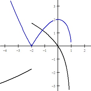
 . Discuss the graph of the relation giving reasons for your conclusions. Include a brief mention of any unproductive paths you followed and what you learned from them.
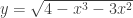 .
. and
and  . What does this say about the graph?
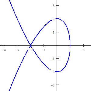
 . Values greater than 1 will make the left side of the equation greater than 4 regardless of the value of y. The range of the relation is all real numbers.
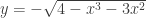
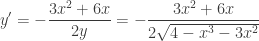 by implicit differentiation or by differentiating the equation for the top half.
 does not exist at x = 1 specifically,
  . Therefore, the line x = 1 is a vertical tangent. By symmetry for the lower part of the graph
  . And x = 1 is its vertical asymptote as well. The slope of the original relation changes from positive to negative at x = 1 by going not through zero but from
  to
to  .
. when x = 0 and when x = –2. At (0, 2) the derivative changes from positive to negative; this is a local maximum point by the first derivative test. The lower half has a local minimum point at (0, –2) by symmetry.
 .
.

 and
and 
 and on the right approaches
  .
.


 , so, substituting
  we have


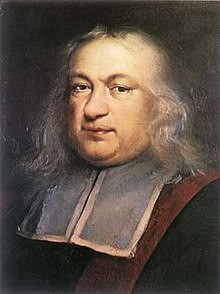
 – Fermat unknowingly is using the derivative! After which he set it equal to 0 and solved to find the
  .
. .
. .
. .
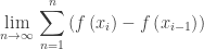
. resembles the right side of the Mean Value Theorem above. Since all the conditions are met, the MVT tells us that in each subinterval
 ![\displaystyle [{{x}_{{i-1}}},{{x}_{i}}]](https://s0.wp.com/latex.php?latex=%5Cdisplaystyle+%5B%7B%7Bx%7D_%7B%7Bi-1%7D%7D%7D%2C%7B%7Bx%7D_%7Bi%7D%7D%5D&bg=ffffff&fg=333333&s=0&c=20201002) there exists a number, call it ci , such that
there exists a number, call it ci , such that and therefore
 – The Fundamental Theorem of Calculus.)
 for all x in the interval. Every function continuous on a closed interval
  for all x in the interval. Every function continuous on a closed interval
  changes sign in the interval, then
  .
.
 is called the remainder. The equation above says that if you can find the correct c the function is exactly equal to Tn(x) + R. Notice the form of the remainder is the same as the other terms, except it is evaluated at the mysterious c. The trouble is we almost never can find the c without knowing the exact value of f(x), but; if we knew that, there would be no need to approximate. However, often without knowing the exact values of c, we can still approximate the value of the remainder and thereby, know how close the polynomial Tn(x) approximates the value of f(x) for values in x in the interval, i. See
 defined on the closed interval [–1,3]
 defined on the closed interval
 ![\left[ {\tfrac{\pi }{2},\tfrac{{9\pi }}{2}} \right]](https://s0.wp.com/latex.php?latex=%5Cleft%5B+%7B%5Ctfrac%7B%5Cpi+%7D%7B2%7D%2C%5Ctfrac%7B%7B9%5Cpi+%7D%7D%7B2%7D%7D+%5Cright%5D&bg=ffffff&fg=333333&s=0&c=20201002)

 defined on the closed interval
 ![\displaystyle [-4.5]](https://s0.wp.com/latex.php?latex=%5Cdisplaystyle+%5B-4.5%5D&bg=ffffff&fg=333333&s=0&c=20201002)


 when x = –1/2, ½, 3/2 and 5/2
 , the slope = 1 at all four points
 and
and  ; the line is

 when
when 
 , at the points above the slope is 1.

 when
when 

