
Seven of nine. This week we continue our look at the 2021 free-response questions with an eye to ways to adapt and expand the questions. Hopefully, you will find ways to use this and other free-response questions to help your students learn more and be better prepared for the exams.
2021 BC 2
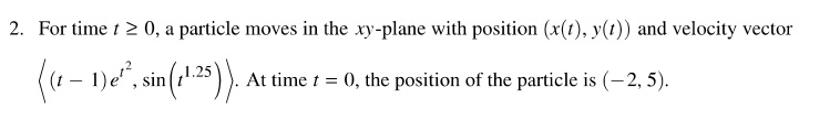
This is a Parametric and Vector Equation (Type 8) question and contains topic from Unit 9 of the current Course and Exam Description. The vector equation of the velocity of a particle moving in the xy-plane is given along with the position of the particle at t = 0. No units were given.
The stem for 2021 BC 2 is next. (Note the 
Part (a): Students were asked to find the speed and acceleration of the particle at t = 1.2. This is a calculator active questions and the students were expected, but not actually required, to use their calculator. With their calculator in parametric mode, students should begin by entering the velocity as xt1(t) and yt1(t).
Discussion and ideas for adapting this question:
- There is little I can suggest here other than changing the time.
- At the given time and other times, you can ask in what direction is the particle moving and which way the acceleration is pulling the velocity.
- Ask student to do this without using their calculator. The answer need not be simplified or expressed as a decimal.
Part (b): Asked the students to find the total distance traveled by the particle over a given the time interval. This must be done on a calculator. Be sure your students know how to enter the expression using the already entered values for xt1(t) and yt1(t). The calculator entry should look like this.

Discussion and ideas for adapting this question:
- Use different intervals.
- Discuss the similarities with the number line distance formula. In linear motion, the distance is simply the integral of the absolute value of the velocity. Since
, this is the same formula reduced to one dimension.
Part (c): The situation is reduced to a one-dimensional problem: students were asked to find the coordinates of the point at which the particle is farthest left and explain why there is no point farthest to the right.
Discussion and ideas for adapting this question:
- Discuss how to do this and how students should present their answer and explanation.
- Show that this is the same as an extreme value problem and done the same way (i.e., find where the derivative is zero, and show that this is a minimum (farthest left), etc.).
- Discuss how you know there is no maximum and interpret this in the context of the equation.
For further exploration. Try graphing the path of the particle. Discuss how to do that with your class. See what they suggest. Here a few approaches.
- The first thought may be to integrate the velocity vector as an initial value problem. Unfortunately, this cannot be done. Neither the x-component nor the y-component can be integrated in terms of Elementary Functions. Even WolframAlpha.com is no help.
- Having entered the velocity vector as xt1(t) and yt1(t), as suggested above, enter something like this depending on your calculator’s syntax and then graph in a suitable window. Compare the graph with the previous analysis in part (c)?


- You may also try expressing the components of velocity as a Taylor series centered at some positive number, a, not at zero. Integrate that to get an approximation to graph. Be sure to adjust things so the initial point is on the graph. WolframAlpha will help here. The one problem here is that the y-component is not defined for negative numbers. Therefore, zero cannt be then center and the largest the interval of convergence can be is [0, 2a] (Why?) and may not even by that large. This is an interesting approach mathematically but will not help with most of the graph.
Personal opinion: I do not think much of this question because all the first two parts require is entering the formula in your calculator and computing the answer, and the third part is really an AB level question. Just my opinion.

Next week 2021 BC 5
I would be happy to hear your ideas for other ways to use this question. Please use the reply box below to share your ideas.

 is to write prominently on their answer page
  and
and  . While they may understand and use this, they must say it.
 by reading the slope of f(x) from the graph.
 may be used. Before assigning your own problem, check that all the values can be found from the given graph.
 equals this value. Students also must justify their answer.
 then the other members of the family are all of the form
  . The c has the same effect as the amplitude of a sine or cosine function:
 and similarly for Q(1). This is a calculator allowed question and students should use their calculator to find the answer and not do it by hand.
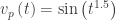 tons per hour for
  hours. At time t = 0 the amount on hand is P = 5 tons.
 tons per hour for
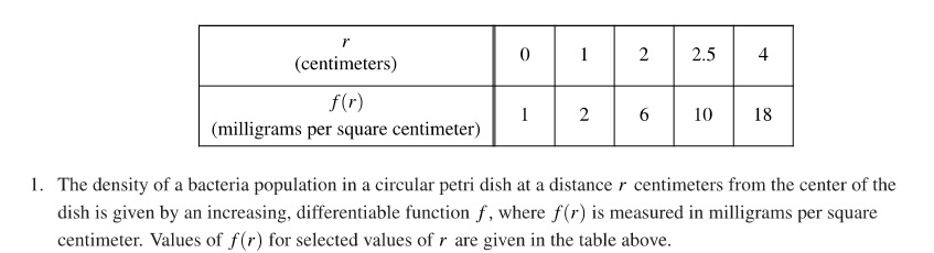
 .
. , but here is a good change to discuss what the units mean. Why does “milligrams per square centimeter per centimeter distant from the center” make more sense?
 , has an “extra” factor of r in it.
 (note “extra” r), the average rate of change on an interval, etc.
 You may change this to explore other graphs. (Because of the way Desmos graphs, you cannot have a slider for θ; the a-slider will move the line and the point on the graph. r(a) gives the value of r(θ).
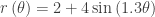 for
for  . This is an area for exploration (if you have time).
  and
and  . This is simple right triangle trigonometry (draw a perpendicular from the point to the x-axis and from there to the pole).
  and
and 

 where
where  from above.
 where
where  from above.
 . See 2018 BC5 (b)
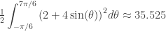
 . This is not the correct area of either part.
  . Between 0 and
  this curve traces the same path twice.