
A Little Calculus is an app for iPad and iPhones. While I don’t usually do product reviews, I think this one is so good that I am making an exception.
There are many good websites that illustrate calculus concepts. Many of them, however, do not allow teachers to enter their own examples; they must use the built-in ones. A Little Calculus is an exception.
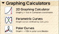
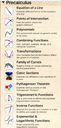
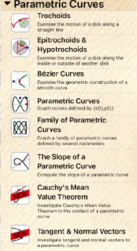
A Little Calculus contains over 75 demonstrations of calculus and calculus related concepts, and also three graphing calculators (Cartesian, Parametric, and Polar). Each demonstration can be fully edited to any function and conditions by the user. The topics cover precalculus, limits and continuity, Differential Calculus, Integral Calculus, Sequences and Series, Parametric Curves, and Multivariable Calculus. A full list of the concepts included is at the end of this post. The app is available in the App Store; the price is (only) $0.99. Link.
Each topic has an information screen (circled I in the upper right of the screen) that includes (1) “How To” explaining how to input your example and how to use the features specific to that demonstration. (You should read this the first time you use each topic because some features may not be obvious.), (2) “Background” a textbook-like page that explains in detail the mathematics demonstrated, and (3) “Examples” discussing one or more examples of the concept.
The set-up screen (chevron upper right) allows the user to enter the example they want. This then changes to a pull-down screen. The screenshot below is the set-up screen for “The Area Under a Curve” demonstration. Note the Riemann rectangles available from the set-up screen.
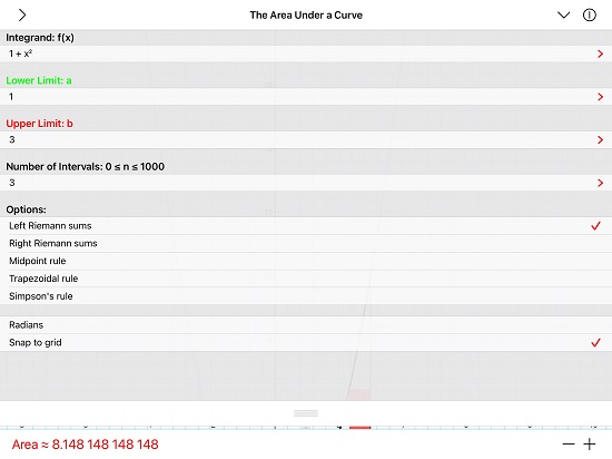
The resulting graph is shown next for 3 right Riemann sum rectangles. By clicking on the “+” or “-“ in the bottom right, you can increase or decrease the number of rectangles one at a time; by holding the “+” sign the number increases rapidly to demonstrate n → ∞. The upper and lower limits may be specified on the set-up screen or be dragged from the graph. The current area of the rectangles is shown in the lower left.

The next illustration shows the “Disk Method” section. The lower graph shows the individual rectangles; the upper shows the 6 rectangles rotated around the line y = –1/2. The “+” button increases the number of rectangles.

This shot shows 150 rectangles; the upper graph has been rotated slightly – this is accomplished in real time by dragging your finger across the screen. All three-dimensional graphs may be moved in this manner.

I could go on …
The one slight drawback is that the input screen does not allow the user to enter parentheses. The parentheses are entered correctly by selecting what is to be enclosed and then tapping the next operation button. This leads to some strange looking expressions such as sin(x)2 instead of (sin(x))2. The expressions are interpreted correctly, but the strange look may confuse some students. It would be easier to type them yourself as usual. Not a big problem.
An effective way to use this app if for the teacher to project a demonstration and discuss the various ideas he or she wishes to discuss. Tapping the screen with two fingers toggles a pointer; this is useful for working on-line with students who cannot see where you are pointing otherwise. Students could use the app to investigate on their own.
UPDATE (August 18,2022) A new feature has been added: you may now save and recall your own example(s) instead of having to reenter them each time. Handy for preparing demonstrations ahead of time or having students prepare their own examples.
Also, two new topics have been added: Logistic growth and the derivative of an exponential function.
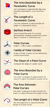
Here is a list of the other topics included:


Update 8-18-2022
 or
or  . Specifically, if a function has a horizontal asymptote(s), then
  , At an asymptote, the curve must approach a horizontal line, therefore its slope must be approaching zero as
 ![\displaystyle f\left( x \right)=\sqrt[3]{x}](https://s0.wp.com/latex.php?latex=%5Cdisplaystyle+f%5Cleft%28+x+%5Cright%29%3D%5Csqrt%5B3%5D%7Bx%7D&bg=ffffff&fg=333333&s=0&c=20201002) .
. (Figure 1 in blue).This is the derivative of
  . (Figure 1 in red). We see that the derivative approaches zero in both directions, this tells us that there may be horizontal asymptote(s). We must look at the function to find where they are:
  and
and 
 since
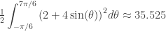
since 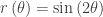 , shown below, appears to show 4 maximums. However, if we trace the graph, we find that these points are (1, π/4), (–1, 3π/4), (1, 5π/4) and (–1, 7π/4). Two of the values are maximums where r(θ) = 1 and two are minimums where r(θ) = –1.
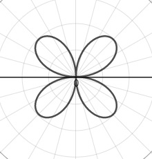

 The domain is extended to
  . Notice:
 You may change this to explore other graphs. (Because of the way Desmos graphs, you cannot have a slider for θ; the a-slider will move the line and the point on the graph. r(a) gives the value of r(θ).
 for
for  and
and  . This is simple right triangle trigonometry (draw a perpendicular from the point to the x-axis and from there to the pole).
  and
and 

 where
where  from above.
 where
where  from above.
 . See 2018 BC5 (b)
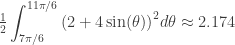
 . This is not the correct area of either part.
  . Between 0 and
  this curve traces the same path twice.
 , sin(x), cos(x), and ex