Tangent Lines

Posted on August 23, 2016 by Lin McMullin

Second in the Graphing Calculator/Technology series

This graphing calculator activity is a way to introduce the idea if the slope of the tangent line as the limit of the slope of a secant line. In it, students will write the equation of a secant line through two very close points. They will then compare their results in several ways.

Begin by having the students graph a very simple curve such as y = x² in the standard window of their calculator. Then TRACE to a point. Students will go to different points, some to the left and some to the right of the origin. ZOOM IN several times on this point until their graph appears linear (discuss local linearity here). To be sure they are on the graph push TRACE again. The coordinates of their point will be at the bottom of the screen; call this point (a, b). Return to the home screen and store the values to A and B (click here for instructions on storing and recalling numbers).

Return to the graph and push TRACE again to be sure the cursor is on the graph. Move the TRACE cursor one or two pixels away from the first point in either direction. This new point is (c, d). Return to the home screen and store the coordinates to C and D.

Enter the equation of the line through the two points on the equation entry screen in terms of A, B, C, and D. Zoom Out several times until you have returned to the original window..

Exploration 1: Have students compare and contrast their graphs with several other students and discuss their observations. (Expected observations: the lines appear tangent at each students’ original point)

Exploration 2: Ask student to compute the slope of the line through their points, again using A, B, C, and D. Collect each student’s x-coordinate, A, and their slope and enter them in list is your calculator so that they can be projected.

Study the two lists and discuss the relation is any. (Expected observations: the slope is twice the x-coordinate.) Can you write an equation of these pairs? (Expected result: y = 2x)

Finally, plot the points on the calculator using a square window. Do the points seem to lie on the line y =2x?

Extensions:

Try the same activity with other functions such as y = (1/3)x³, y = x³, or y = x⁴. Anything more difficult will still result in a tangent line, but the numerical relationship between x and the slope will probably be too difficult to see. You may also consider y = sin(x) or y = cos(x). Again, the numerical work in Exploration 2, will be too difficult to see, but on graphing the points the result may be obvious. For y = sin(x), return to the list and add a column with the cosines of the x-values. Compare these with the slopes.

Using the Derivative to Graph the Function

Posted on September 9, 2015 by Lin McMullin

In my last post I showed how to use a Desmos graph to discover, by looking at the tangent line as it moved along the graph of the function, the properties of the derivative of a function. This post goes in the opposite direction. Now, instead of discovering the properties of the derivative from the graph of the function, we will use that knowledge to identify important information about the function from the graph of its derivative. We are not discovering anything here; rather we are putting our previous discoveries to use.

One of the uses of the derivative is to deduce properties of its antiderivative, i.e. the function of which it is the derivative. This is an important skill for students to be able to use. It is also a type of question that appears on every Advanced Placement Calculus exam in both the free-response sections and the multiple-choice sections. My previous post on this topic, Reading the Derivative’s Graph, is the most read post on this blog. This post expands on the concepts in that post and shows how to use the Desmos file to help students develop the skills necessary to answer this type of question.

Desmos is free. You and your students can set up their own account and save their own work there. There are also free Desmos apps for tablets and smart phones.

Click on the graph above. Here’s what you should see:

The first equation on the left side is f(x). This is the function whose antiderivative we will be trying to create. You may change this to any function you wish.
The second equation is F(x) the antiderivative of f(x). That is F ‘(x) = f(x). Desmos cannot compute an antiderivative so you will need to enter it yourself. Your students need not trust you on this: have them check your equation by differentiating. Of course, at this point they will not be ready to find the analytic form of the antiderivative except for the simplest functions. This comes later in the year.
Note the “+C” is included and later we will manipulate this with a slider.
The antiderivative is multiplied by $\frac{\sqrt{a-x}}{\sqrt{a-x}}$ . This is a way of controlling the “a” slider and should always be multiplied by antiderivative. This is just a syntax trick to make the graph work and is not part of the antiderivative. When x is to the left of a, (x < a) the fraction is 1 and the graph will be seen; when x is to the right of a, (x > a) the expression is undefined, and nothing will graph. As you change “a” with the slider the graph of an antiderivative will be drawn.
The third equation x = a graphs a dashed vertical to help you line up the corresponding points on the two graphs.
The next two lines are the “a” and “C” sliders. Make C = 0 for now and move the “a” slider.

At this point students should know things about the relationship between a function and its first and second derivatives. This includes the things they discovered in the previous post such as when the function is increasing the derivative is non-negative, and when the tangent line is above the graph the slope (derivative) is decreasing and the graph of the function is concave down. All of these concepts are really “if, and only if” situations. So we now consider them in reverse and deduce properties of the antiderivative from the properties of the graph of the derivative.

Using the “a” slider starting at the left side of the graph ask the students what the derivative tells them about the function in this part of the domain. Is the function increasing or decreasing? Is it concave up or down? etc. Go slowly from left to right asking what happens next, and why (that is, how do you know? What feature of the derivative tells you this?) This is preparing them to write the justifications required on the AP exams.

Certain points on the graph of the derivative are important. The zeros of the derivative and whether the derivative changes from positive to negative, negative to positive, or neither are important. Likewise, the extreme values of the derivative point to important features of the function – points of inflection.

Once you have a complete graph of the antiderivative move the “C” slider.

Remind students that the derivative of a constant is zero and therefore, the C does not show up in the derivative.
Discuss is why changing the antiderivative does not change the derivative.
Ask, how many functions have the same derivative?
Point out is that by changing “C” the graph of an antiderivative can be made to go through any (every, all) point in the plane.

Switch to a different function and its derivative to reinforce the concepts. Yo will have to enter both the derivative and the antiderivative.Do this as often as necessary. You could also give students or groups of students the graph of a derivative (on paper) and challenge them to sketch the antiderivative.

A disclaimer: A function and its derivative should not be graphed on the same axes, because the two have different units. Nevertheless, I have done it here, and it is commonly done everywhere, to compare the graphs of a function and its derivative so that the important features of the two can be lined up and easily compared.

Good Question 1: 2008 AB 6

Posted on January 21, 2015 by Lin McMullin

When I started this blog several years ago I was hoping my readers would ask questions that we could discuss or submit ideas for additional topics to write about. This has not really happened, but I’m still very open to the idea. (That was a HINT.) Since that first year when I had the entire curriculum ahead of me, I have written less not because I dislike writing, but because I am low on ideas.

The other day, I answered a question posted on the AP Calculus Community bulletin board about AB calculus exam question. It occurred to me that this somewhat innocuous looking question was quite good. So I decided to start an occasional series on good questions, from AP exams or elsewhere, that can be used to teaching beyond the actual things asked in the question. (My last post might be in this category, but that was written several months ago.)

In discussing these questions, I will make numerous comments about the question and how to take it further in your class. My idea is not just to show how to write a good answer, but rather to use the question to look deeper into the concepts involved.

Good Question #1: 2008 AB Calculus exam question 6.

The stem gave students the function $\displaystyle f\left( x \right)=\frac{\ln \left( x \right)}{x},\quad x>0$ . Students were also told that $\displaystyle {f}'\left( x \right)=\frac{1-\ln \left( x \right)}{{{x}^{2}}}$ .

The first thought that occurs is why they gave the derivative. The reason is, as we will see, that the first derivative is necessary to answer the first three parts of the question. Therefore, a student who calculates an incorrect derivative is going to be in big trouble (and the readers may have a great deal of work to do reading with the student’s incorrect work). The derivative is calculated using the quotient rule, and students will have to demonstrate their knowledge of the quotient rule later in this question; there is no reason to ask them to do the same thing twice.
If you are using this with a class, you can, and probably should, ask your students to calculate the first derivative. Then you can see how many giving the derivative would have helped.
When discussing the stem, you should also discuss the domain, x > 0, and the x-intercept (1, 0). Other features of the graph, such as end behavior, are developed later in the question, so they may be put on hold briefly.

Part a asked students to write an equation of the tangent line at x = e². To do this students need to do two calculations: $\displaystyle f\left( {{e}^{2}} \right)=\frac{2}{{{e}^{2}}}$ and $\displaystyle {f}'\left( {{e}^{2}} \right)=-\frac{1}{{{e}^{4}}}$ . An equation of the tangent line is $\displaystyle y=\frac{2}{{{e}^{2}}}-\frac{1}{{{e}^{4}}}\left( x-{{e}^{2}} \right)$ .

Writing the equation of a tangent line is a very important skill and should be straightforward. The point-slope form is the way to go. Avoid slope-intercept.
The tangent line is used to approximate the value of the function near the point of tangency; you can throw in an approximation computation here.
After doing part c, you should return here and discuss whether the approximation is an overestimate or an underestimate and how you can tell. (Answer: underestimate, since the graph is concave up here.)
After doing part c, you can also ask them to write the tangent line at the point of inflection and whether approximations near the point of inflection are overestimates or an underestimates, and why. (Answer: Since the concavity change here, it depends on which side of the point of inflection the approximation is made. To the left is an overestimate; to the right is an underestimate.)

Part b asked students to find the x-coordinate of the critical point, determine whether it is a maximum, a minimum, or neither, and to “justify your answer.” To earn credit students had to write the equation $\displaystyle {f}'\left( x \right)=0$ and solve it getting x = e. They had to state that this is a maximum because “ ${f}'\left( x \right)$ changes from positive to negative at x = e.”

This is a very standard AP exam question. To expand it in your class:

Discuss how you know the derivative changes sign here. This will get you into the properties of the natural logarithm function.
Discuss why the change in sign tells you this is a maximum. (A positive derivative indicates an increasing function, etc.)
After doing part c, you can return here and try the second derivative test.
The question asks for “the” critical point, hinting that there is only one. Students should learn to pick up on hints like this and be careful if their computation produces more or less than one.
At this point we have also determined that the function is increasing on the interval $\left( -\infty ,e \right]$ and decreasing everywhere else. The question does not ever ask this, but in class this is worth discussing as important features of the graph. On why these are half-open intervals look here.

Part c told students there was exactly one point of inflection and asked them to find its x-coordinate. To do this they had to use the quotient rule to find that $\displaystyle {{f}'}'\left( x \right)=\frac{-3+2\ln \left( x \right)}{{{x}^{3}}}$ , set this equal to zero and find the x-coordinate to be x = e^3/2.

The question did not require any justification for this answer. In class you should discuss what a justification would look like. The reason is that the second derivative changes sign here. So now you need to discuss how you know this.
Also, you can now determine that the function is concave down on the interval $\left( -\infty ,{{e}^{3/2}} \right)$ and concave up on the interval $\left({{e}^{3/2}},\infty \right)$ . Ask your class to justify this.

Part d asked student to find $\displaystyle \underset{x\to 0+}{\mathop{\lim }}\,\frac{\ln \left( x \right)}{x}$ . The answer is $-\infty$ . While this seems almost like a throwaway tacked on the end because they needed another point, it is the reason I like this question.

The question is easily solved: $\displaystyle \underset{x\to 0+}{\mathop{\lim }}\,\frac{\ln \left( x \right)}{x}=\underset{x\to 0+}{\mathop{\lim }}\,\frac{1}{x}\cdot \underset{x\to 0+}{\mathop{\lim }}\,\ln \left( x \right)=\left( \infty \right)\left( -\infty \right)=-\infty$ .
While tempting, the limit cannot be found by L’Hôpital’s Rule, because on substitution you get $\frac{-\infty }{0}$ ,which is not one of the forms that L’Hôpital’s Rule can handle.
The reason I like this part so much is that we have already developed enough information in the course of doing the problem to find this limit! The function is increasing and concave down on the interval $\left( -\infty ,e \right)$ . Moving from the maximum to the left, the function crosses the x-axis at (1, 0), keeps heading south, and gets steeper. So the limit as you approach the y-axis from the right is negative infinity.This is the left-side end behavior.
What about the right-side end behavior? (You ask your class.) Well, the function is positive and decreasing to the right of the maximum and becomes concave up after x = e^3/2. Thus, it must flatten out and approach the x-axis as an asymptote.
That $\displaystyle \underset{x\to \infty }{\mathop{\lim }}\,\frac{\ln \left( x \right)}{x}=0$ is clear from the note immediately above. This limit can be found by L’Hôpital’s Rule since it is an indeterminate of the type $\infty /\infty$ . So, $\displaystyle \underset{x\to \infty }{\mathop{\lim }}\,\frac{\ln \left( x \right)}{x}=\underset{x\to \infty }{\mathop{\lim }}\,\frac{\tfrac{1}{x}}{1}=0$ .
Notice also that the first derivative approaches zero as x approaches infinity. This indicates that the function’s graph approaches the horizontal as you travel farther to the right. The second derivative also approaches zero as x approaches infinity indicating that the function’s graph is becoming flatter (less concave).

This question and the discussion is largely done analytically (working with equations). We did find a few important numbers in the course of the work. Hopefully, you students discussed this with many good words. To complete the Rule of Four, here is the graph.

And here is a close up showing the important features of the graph and the corresponding points on the derivatives.

The function is shown in blue, the derivative and maximum in red, and the second derivative and the point of inflection in green.

Finally, this function and the limit at infinity is similar to the more pathological example discussed in the post of October 31, 2012 entitled Far Out!

Darboux’s Theorem

Posted on August 18, 2014 by Lin McMullin

Jean Gaston Darboux
1842 – 1917

Jean Gaston Darboux was a French mathematician who lived from 1842 to 1917. Of his several important theorems the one we will consider says that the derivative of a function has the Intermediate Value Theorem property – that is, the derivative takes on all the values between the values of the derivative at the endpoints of the interval under consideration.

Darboux’s Theorem is easy to understand and prove but is not usually included in a first-year calculus course (and is not included on the AP exams). Its use is in the more detailed study of functions in a real analysis course.

You may want to use this as an enrichment topic in your calculus course, or a topic for a little deeper investigation. The ideas here are certainly within the range of what first-year calculus students should be able to follow. They relate closely to the Mean Value Theorem (MVT). I will suggest some ideas (in blue) to consider along the way.

More precisely Darboux’s theorem says that

If f is differentiable on the closed interval [a, b] and r is any number between f ’ (a) and f ’ (b), then there exists a number c in the open interval (a, b) such that f ‘ (c) = r.

Differentiable on a closed interval?

Most theorems in beginning calculus require only that the function be differentiable on an open interval. Here, obviously, we need a closed interval so that there will be values of the derivative for r to be between.

The limit definition of derivative requires a regular two-sided limit to exist; at the endpoint of an interval there is only one side. For most theorems this is enough. Here the definition of derivative must be extended to allow one-sided limits as x approaches the endpoint values from inside the interval. Also note that if a function is differentiable on (a, b), then it is differentiable on any closed sub-interval of (a, b) that does not include a or b.

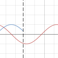
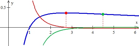
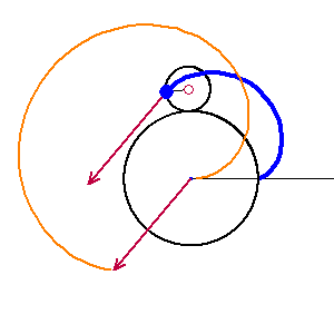
Geometric proof [1]

Consider the diagram below, which shows a function in blue. At each endpoint draw a line with the slope of r. Notice that these two lines have a slope less than that of the function at the left end and greater than the slope at the right end. At least one of these lines must intersect the function at an interior point of the interval. Before reading on, see if you and your students can complete the proof from here. (Hint: What theorem does the top half of the figure remind you of?)

On the interval between the intersection point and the end point we can apply the Mean Value Theorem and determine the value of c where the tangent line will be parallel to the line through the endpoint. At this point f ‘(c) = r. Q.E.D.

Analytic Proof [2]

Consider the function $h\left( x \right)=f\left( x \right)-(f(b)+r(x-b))$ . Since f(x) is differentiable, it is continuous; $\displaystyle f(b)+r(x-a)$ is also continuous and differentiable. Therefore, h(x) is continuous and differentiable on [a, b]. By the Extreme Value Theorem, there must be a point, x = c, in the open interval (a, b) where h(x) has an extreme value. At this point h’ (c) = 0.

Before reading on see if you can complete the proof from here.

$\displaystyle h(x)=f(x)-(f(b)+r(x-a))$

$\displaystyle {h}'(x)={f}'(x)-r$

$\displaystyle {h}'(c)={f}'(c)-r=0$

$\displaystyle {f}'\left( c \right)=r$

Q.E.D.

Exercise: Compare and contrast the two proofs.

In the geometric proof, what does $\displaystyle y=f(b)+r(x-a)$ represent? Where does it show up in the diagram?
How do both proofs relate to the Mean Value Theorem (or Rolle’s Theorem).

The function $\displaystyle h(x)=f(x)-(f(b)+r(x-a))$ represents the vertical distance from f(x) to $\displaystyle f(b)+r(x-a)$ . In the diagram, this is a vertical segment connecting f(x) to $\displaystyle y=f(b)+r(x-a)$ .This expression may be positive, negative, or zero. In the diagram, at the point(s) where the line through the right endpoint intersects the curve and at the endpoint h(x) = 0. Therefore, h(x) meets the hypotheses of Rolle’s Theorem (and the MVT), and the result follows.

The line through the right endpoint will have equation the $y=f(b)+r(x-b)$ This makes $h\left( x \right)=f\left( x \right)-\left( f(b)+r(x-b) \right)$ . When differentiated and the result will be ${f}'\left( x \right)-r$ the same expression as in the analytic proof.

Also, you may move this line upwards parallel to its original position and eventually it will be tangent to the graph of the function. (See my posts on MVT 1 and especially MVT 2).

Exercise:

Consider the function f(x) = sin(x)

On the interval [1,3] what values of the derivative of f are guaranteed by Darboux’s Theorem? .
Does Darboux’s theorem guarantee any value on the interval $[0,2\pi ]$ ? Why or why not?

Answers:

f ‘(x) = cos(x). f ‘ (1) = 0.54030 and f ‘ (3) = -0.98999. So the guaranteed values are from -0.98999 to 0.54030.
No. f ‘ (x) = 1 at both endpoints, so there are no values between one and one.

Another interesting aspect of Darboux’s Theorem is that there is no requirement that the derivative f ‘(x) be continuous!

A common example of such a function is

$\displaystyle f\left( x \right)=\left\{ \begin{matrix} {{x}^{2}}\sin \left( \frac{1}{x} \right) & x\ne 0 \\ 0 & x=0 \\ \end{matrix} \right.$

With $\displaystyle {f}'\left( x \right)=-\cos \left( \tfrac{1}{x} \right)+2x\sin \left( \tfrac{1}{x} \right),\,\,x\ne 0$ .

This function (which has appeared on the AP exams) is differentiable (and therefore continuous).There is an oscillating discontinuity at the origin. The derivative is not continuous at the origin. Yet, every interval containing the origin as an interior point meets the conditions of Darboux’s Theorem, so the derivative while not continuous has the intermediate value property.

AP exam question 1999 AB3/BC3 part c:

Finally, what inspired this post was a recent discussion on the AP Calculus Community bulletin board about the AP exam question 1999 AB3/BC3 part c. This question gave a table of values for the rate, R, at which water was flowing out of a pipe as a differentiable function of time t. The question asked if there was a time when R’ (t) = 0. It was expected that students would use Rolle’s Theorem or the MVT. There was a discussion about using Darboux’s theorem or saying something like the derivative increased (or was positive), then decreased (was negative) so somewhere the derivative must be zero (implying that derivative had the intermediate value property). Luckily, no one tried this approach, so it was a moot point.

Take a look at the problem with your students and see if you can use Darboux’s theorem. Be sure the hypotheses are met.

Answer (try it yourself before reading on):

The function is not differentiable at the endpoints. But consider an interval like [0,3]. Using the given values in the table, by the MVT there is a time t = c where R‘(c) = 0.8/3 > 0, and there is a time t = d on the interval [21, 24] where R‘(d) = -0.6/3 < 0. The function is differentiable on the closed interval [c, d] so by Darboux’s Theorem there must exist a time when R’(t) = 0. Admittedly, this is a bit of overkill.

References:

After Nitecki, Zbigniew H. Calculus Deconstructed A Second Course in First-Year Calculus, ©2009, The Mathematical Association of America, ISBN 978-0-883835-756-4, p. 221-222.
After Dunham, William The Calculus Gallery Masterpieces from Newton to Lebesque, © 2005, Princeton University Press, ISBN 978-0-691-09565-3, p. 156.

Both these book are good reference books.

Updated: August 20, 2014, and October 4, 2017

Roulettes and Calculus

Posted on July 11, 2014 by Lin McMullin

Roulettes – 5: Calculus Considerations.

In the first post of this series Roulette Generators (RG) are explained. Here are the files for Winplot or Geometer’s Sketchpad. Use them to quickly see the graphs of these curves by adjusting one or two parameters.

While writing this series of posts I was intrigued by the cusps that appear in some of the curves. In Cartesian coordinates you think of a cusp as a place where the curves is continuous, but the derivative is undefined, and the tangent line is vertical. Cusps on the curves we have been considering are different.

The equations of the curves formed by a point attached to a circle rolling around a fixed circle in the form we have been using are:

$x\left( t \right)=(1+R)\cos \left( t \right)-S\cos \left( \tfrac{1}{R}t+t \right)$

$y\left( t \right)=\left( 1+R \right)\sin \left( t \right)-S\sin \left( \tfrac{1}{R}t+t \right)$

For example, let’s consider the case with $R=S=\tfrac{1}{3}$

Epicycloid with R = S = 1/3

The equations become

$x\left( t \right)=\frac{4}{3}\cos \left( t \right)-\frac{1}{3}\cos \left( 4t \right)$

$y\left( t \right)=\frac{4}{3}\sin \left( t \right)-\frac{1}{3}\sin \left( 4t \right)$

The derivative is

$\displaystyle \frac{dy}{dx}=\frac{dy/dt}{dx/dt}=\frac{\cos \left( t \right)-\cos (4t)}{-\sin \left( t \right)+\sin (4t)}$

The cusps are evenly spaced one-third of the way around the circle and appear at $t=0,\tfrac{2\pi }{3},\tfrac{4\pi }{3}$ . At the cusps dy/dx is an indeterminate form of the type 0/0. (Note that at $t=\tfrac{2\pi }{3}$ , $\cos \left( 4t \right)=\cos \left( \tfrac{8\pi }{3} \right)=\cos \left( \tfrac{2\pi }{3} \right)$ and likewise for the sine.) Since derivatives are limits, we can apply L’Hôpital’s Rule and find that at $t=\tfrac{2\pi }{3}$

$\displaystyle \frac{dy}{dx}=\underset{t\to \tfrac{2\pi }{3}}{\mathop{\lim }}\,\frac{-\sin \left( t \right)+4\sin \left( 4t \right)}{-\cos \left( t \right)+4\cos \left( 4t \right)}=\underset{t\to \tfrac{2\pi }{3}}{\mathop{\lim }}\,\frac{3\sin \left( t \right)}{3\cos \left( t \right)}=\tan \left( \tfrac{2\pi }{3} \right)=-\sqrt{3}$

This is, I hope, exactly what we should expect. As the curve enters and leaves the cusp it is tangent to the line from the cusp to the origin. (The same thing happens at the other two cusps.) At the cusps the moving circle has completed a full revolution and thus, the line from its center to the center of the fixed circle goes through the cusp and has a slope of tan(t).

The cusps will appear where the same t makes dy/dt = 0 and dx/dt =0 simultaneously.

The parametric derivative is defined at the cusp and is the slope of the line from the cusp to the origin. Now I may get an argument on that, but that’s the way it seems to me.

A look at the graph of the derivative in parametric form may help us to see what is going on. In the next figure $R=S=\tfrac{1}{3}$ with the graph of the curve is in blue. The velocity vector is shown twice (arrows). The first is attached to the moving point and shows the direction and its length shows the speed of the movement. The second shows the velocity vector as a position vector (tail at the origin). The orange graph is the path of the velocity vector’s tip – the parametric graph of the velocity. Note that these vectors are the same (i.e. they have the same direction and magnitude)

The video shows the curve moving through the cusp at. Notice that as the graph passes through the cusp the velocity vector changes from pointing down to the right, to the zero vector, to pointing up to the left. The change is continuous and smooth.

Velocity near a cusp.

Here is the whole curve being drawn with its velocity and the velocity vectors.

Epicycloid with velocity vectors

(If you are using the Winplot file you graph the velocity this way. Open the inventory with CTRL+I, scroll down to the bottom and select, one at a time, the last three lines marked “hidden”, and then click on “Graph.”). The Geometer’s Sketchpad version has a button to show the derivative’s graph and the velocity vectors.

The general equation of the derivative (velocity vector) is

$\displaystyle {x}'\left( t \right)=-\left( 1+R \right)\sin \left( t \right)+S\left( \tfrac{1}{R}+1 \right)\sin \left( \tfrac{1}{R}t+t \right)$

$\displaystyle {y}'\left( t \right)=\left( 1+R \right)\cos \left( t \right)-S\left( \tfrac{1}{R}+1 \right)\cos \left( \tfrac{1}{R}t+t \right)$

Notice that the derivative has to same form as a roulette.

Finally, I have to mention how much seeing the graphs in motion have helped me understand, not just the derivatives, but all of the curves in this series and the ones to come. To experiment, to ask “what if … ?” questions, and just to play is what technology should be used for in the classroom. See what your students can find using the RGs.

Exploration and Challenge:

Consider the epitrochoid $x\left( t \right)=\frac{2}{3}\cos \left( t \right)+\frac{1}{3}\cos \left( 2t \right),y\left( t \right)=\frac{2}{3}\sin \left( t \right)-\frac{1}{3}\sin \left( 2t \right)$ .

Find its derivative as a parametric equation and graph it with a graphing program or calculator. (Straight forward)
Are the graph of the derivative and the graph of the rose curve given in polar form by $r\left( t \right)=\frac{4}{3}\sin \left( 3t \right)$ the same? Justify your answer. (Warning: The graphs certainly look the same. I have not been able to do show they are the same (which certainly doesn’t prove anything), so they may not be the same.) Please post your answer using the “Leave a Reply” box at the end of this post.

Next: Roulette Art.

Implicit Differentiation of Parametric Equations

Posted on May 17, 2014 by Lin McMullin

I’ve never liked memorizing formulas. I would rather know where they came from or be able to tie it to something I already know. One of my least favorite formulas to remember and explain was the formula for the second derivative of a curve given in parametric form. No longer.

If $y=y\left( t \right)$ and, $x=x\left( t \right)$ then the tradition formula gives

$\displaystyle \frac{d}{dx}y\left( t \right)=\frac{dy/dt}{dx/dt}$ , and

$\displaystyle \frac{{{d}^{2}}y}{d{{x}^{2}}}=\frac{\frac{d}{dt}\left( \frac{dy}{dx} \right)}{\frac{dx}{dt}}$

It is that last part, where you divide by $\displaystyle \frac{dx}{dt}$ , that bothers me. Where did the $\displaystyle \frac{dx}{dt}$ come from?

Then it occurred to me that dividing by $\displaystyle \frac{dx}{dt}$ is the same as multiplying by $\displaystyle \frac{dt}{dx}$

It’s just implicit differentiation!

Since $\displaystyle \frac{dy}{dx}$ is a function of t you must begin by differentiating the first derivative with respect to t. Then treating this as a typical Chain Rule situation and multiplying by $\displaystyle \frac{dt}{dx}$ gives the second derivative. (There is a technical requirement here that given $x=x\left( t \right)$ , then $t={{x}^{-1}}\left( x \right)$ exists.)

In fact, if you look at a proof of the formula for the first derivative, that’s what happens there as well:

$\displaystyle \frac{d}{dx}y\left( t \right)=\frac{dy}{dt}\cdot \frac{dt}{dx}=\frac{dy/dt}{dx/dt}$

The reason you to do it this way is that since x is given as a function of t, it may be difficult to solve for t so you can find dt/dx in terms of x. But you don’t have to; just divide by dx/dt which you already know.

Here is an example for both derivatives.

Suppose that $x={{t}^{3}}-3$ and $y=\ln \left( t \right)$

Then $\displaystyle \frac{dy}{dt}=\frac{1}{t}$ , and $\displaystyle \frac{dx}{dt}=3{{t}^{2}}$ and $\displaystyle \frac{dt}{dx}=\frac{1}{3{{t}^{2}}}$ .

Then $\displaystyle \frac{dy}{dx}=\frac{1}{t}\cdot \frac{dt}{dx}=\frac{1}{t}\cdot \frac{1}{3{{t}^{2}}}=\frac{1}{3{{t}^{3}}}=\frac{1}{3}{{t}^{-3}}$

And $\displaystyle \frac{{{d}^{2}}y}{d{{x}^{2}}}=\left( \frac{d}{dt}\left( \frac{dy}{dx} \right) \right)\cdot \frac{dt}{dx}=\left( -{{t}^{-4}} \right)\cdot \frac{dt}{dx}=\left( -{{t}^{-4}} \right)\left( \frac{1}{3{{t}^{2}}} \right)=-\frac{1}{3{{t}^{6}}}$

Yes, it’s the same thing as using the traditional formula, but now I’ll never have to worry about forgetting the formula or being unsure how to explain why you do it this way.

Revised: Correction to last equation 5/18/2014

Revised: 2/8/2016

Foreshadowing the Chain Rule

Posted on September 20, 2013 by Lin McMullin

I assigned another very easy but good problem this week. It was simple enough, but it gave a hint of things to come.

Use the Product Rule to find the derivative of ${{\left( f\left( x \right) \right)}^{2}}$ .

Since we have not yet discussed the Chain Rule, the Product Rule was the only way to go.

$\frac{d}{dx}{{\left( f \right)}^{2}}=\frac{d}{dx}\left( f\cdot f \right)=f\cdot {f}'+{f}'\cdot f=2f\cdot f'$

And likewise for higher powers:

$\frac{d}{dx}{{f}^{3}}=\frac{d}{dx}\left( f\cdot f\cdot f \right)=f\cdot f\cdot {f}'+f\cdot {f}'\cdot f+{f}'\cdot f\cdot f=3{{f}^{2}}{f}'$

If you just look at the answer, it is not clear where the ${f}'$ comes from. But the result foreshadows the Chain Rule.

Then we used the new formula to differentiate a few expressions such as ${{\left( 4x+7 \right)}^{2}}$ and ${{\sin }^{2}}\left( x \right)$ and a few others.

Regarding the Chain Rule: I have always been a proponent of the Rule of Four, but I have never seen a good graphical explanation of the Chain Rule. (If someone has one, PLEASE send it to me – I’ll share it.)

Here is a rough verbal explanation that might help a little.

Consider the graph of $y=\sin \left( x \right)$ . On the interval $[0,2\pi ]$ it goes through all its value in order once – from 0 to 1 to 0 to -1 and back to zero. Now consider the graph of $y=\sin \left( 3x \right)$ . On the interval $\left[ 0,\tfrac{2\pi }{3} \right]$ it goes through all the same values in one-third of the time. Therefore, it must go through them three times as fast. So the rate of change of $y=\sin \left( 3x \right)$ between 0 and $\tfrac{2\pi }{3}$ must be three times the rate of change of $y=\sin \left( x \right)$ . So the rate of change of must be $3\cos \left( 3x \right)$ . Of course this rate of change is the slope and the derivative.