Roulettes and Calculus

Roulettes – 5: Calculus Considerations.

In the first post of this series Roulette Generators (RG) are explained. Here are the files for Winplot or Geometer’s Sketchpad. Use them to quickly see the graphs of these curves by adjusting one or two parameters.

While writing this series of posts I was intrigued by the cusps that appear in some of the curves. In Cartesian coordinates you think of a cusp as a place where the curves is continuous, but the derivative is undefined, and the tangent line is vertical. Cusps on the curves we have been considering are different.

The equations of the curves formed by a point attached to a circle rolling around a fixed circle in the form we have been using are:

x\left( t \right)=(1+R)\cos \left( t \right)-S\cos \left( \tfrac{1}{R}t+t \right)

y\left( t \right)=\left( 1+R \right)\sin \left( t \right)-S\sin \left( \tfrac{1}{R}t+t \right)

For example, let’s consider the case with R=S=\tfrac{1}{3}


Epicycloid with R = S = 1/3

Epicycloid with R = S = 1/3

The equations become

x\left( t \right)=\frac{4}{3}\cos \left( t \right)-\frac{1}{3}\cos \left( 4t \right)

y\left( t \right)=\frac{4}{3}\sin \left( t \right)-\frac{1}{3}\sin \left( 4t \right)

The derivative is

\displaystyle \frac{dy}{dx}=\frac{dy/dt}{dx/dt}=\frac{\cos \left( t \right)-\cos (4t)}{-\sin \left( t \right)+\sin (4t)}

The cusps are evenly spaced one-third of the way around the circle and appear at t=0,\tfrac{2\pi }{3},\tfrac{4\pi }{3}. At the cusps dy/dx is an indeterminate form of the type 0/0. (Note that at t=\tfrac{2\pi }{3}\cos \left( 4t \right)=\cos \left( \tfrac{8\pi }{3} \right)=\cos \left( \tfrac{2\pi }{3} \right) and likewise for the sine.) Since derivatives are limits, we can apply L’Hôpital’s Rule and find that at t=\tfrac{2\pi }{3}

\displaystyle \frac{dy}{dx}=\underset{t\to \tfrac{2\pi }{3}}{\mathop{\lim }}\,\frac{-\sin \left( t \right)+4\sin \left( 4t \right)}{-\cos \left( t \right)+4\cos \left( 4t \right)}=\underset{t\to \tfrac{2\pi }{3}}{\mathop{\lim }}\,\frac{3\sin \left( t \right)}{3\cos \left( t \right)}=\tan \left( \tfrac{2\pi }{3} \right)=-\sqrt{3}

This is, I hope, exactly what we should expect. As the curve enters and leaves the cusp it is tangent to the line from the cusp to the origin. (The same thing happens at the other two cusps.)  At the cusps the moving circle has completed a full revolution and thus, the line from its center to the center of the fixed circle goes through the cusp and has a slope of tan(t).

The cusps will appear where the same t makes dy/dt = 0 and dx/dt =0 simultaneously.

The parametric derivative is defined at the cusp and is the slope of the line from the cusp to the origin. Now I may get an argument on that, but that’s the way it seems to me.

A look at the graph of the derivative in parametric form may help us to see what is going on. In the next figure R=S=\tfrac{1}{3} with the graph of the curve is in blue. The velocity vector is shown twice (arrows). The first is attached to the moving point and shows the direction and its length shows the speed of the movement. The second shows the velocity vector as a position vector (tail at the origin). The orange graph is the path of the velocity vector’s tip – the parametric graph of the velocity. Note that these vectors are the same (i.e. they have the same direction and magnitude)

The video shows the curve moving through the cusp at. Notice that as the graph passes through the cusp the velocity vector changes from pointing down to the right, to the zero vector, to pointing up to the left. The change is continuous and smooth.

Velocity near a cusp.

Velocity near a cusp.

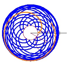
Here is the whole curve being drawn with its velocity and the velocity vectors.

Epicycloid with velocity vectors

Epicycloid with velocity vectors

(If you are using the Winplot file you graph the velocity this way. Open the inventory with CTRL+I, scroll down to the bottom and select, one at a time, the last three lines marked “hidden”, and then click on “Graph.”). The Geometer’s Sketchpad version has a button to show the derivative’s graph and the velocity vectors.

The general equation of the derivative (velocity vector) is

\displaystyle {x}'\left( t \right)=-\left( 1+R \right)\sin \left( t \right)+S\left( \tfrac{1}{R}+1 \right)\sin \left( \tfrac{1}{R}t+t \right)

\displaystyle {y}'\left( t \right)=\left( 1+R \right)\cos \left( t \right)-S\left( \tfrac{1}{R}+1 \right)\cos \left( \tfrac{1}{R}t+t \right)

Notice that the derivative has to same form as a roulette.

Finally, I have to mention how much seeing the graphs in motion have helped me understand, not just the derivatives, but all of the curves in this series and the ones to come. To experiment, to ask “what if … ?” questions, and just to play is what technology should be used for in the classroom. See what your students can find using the RGs.

Exploration and Challenge:

Consider the epitrochoid x\left( t \right)=\frac{2}{3}\cos \left( t \right)+\frac{1}{3}\cos \left( 2t \right),y\left( t \right)=\frac{2}{3}\sin \left( t \right)-\frac{1}{3}\sin \left( 2t \right).

  1. Find its derivative as a parametric equation and graph it with a graphing program or calculator. (Straight forward)
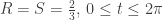
  2. Are the graph of the derivative and the graph of the rose curve given in polar form by r\left( t \right)=\frac{4}{3}\sin \left( 3t \right) the same? Justify your answer.  (Warning: The graphs certainly look the same. I have not been able to do show they are  the same (which certainly doesn’t prove anything), so they may not be the same.) Please post your answer using the “Leave a Reply” box at the end of this post.

Next: Roulette Art.


Advertisement

Hypocycloids and Hypotrochoids

Roulettes – 4: Hypocycloids and Hypotrochoids

In our last few posts we investigated rouletts, the curves that are formed by the locus of points attached to a circle as it rolls around the outside of a fixed circle. Depending on the ratio of the radii (and therefore the circumferences) of the circles these curves are the cardiods (equal radii), epicycloids (moving circle’s radius is less than the fixed circle), and epitrochoids (the point is in the interior or exterior of the moving circle).

In the first post of this series Roulette Generators are explained. Here are the files for Winplot or Geometer’s Sketchpad. Use them to quickly see the graphs of these curves by adjusting one or two parameters.

The parametric equations of these curves are below. and S are parameters that are adjusted for each curve.

x\left( t \right)=(1+R)\cos \left( t \right)-S\cos \left( \tfrac{1}{R}t+t \right)

y\left( t \right)=\left( 1+R \right)\sin \left( t \right)-S\sin \left( \tfrac{1}{R}t+t \right)

We shall now consider the curves that result when the moving circle rolls around the inside of the fixed circle. These curves are called hypocycloids and hypotrochoids. To generate today’s curves make the radius, R, of the moving circle negative.

The first seems almost a special case. Let R =  – 0.5 and S = 0.5 (below left) and then let R = S = – 0.5 (below right). The results are segments, which as we shall see are actually degenerate ellipses.

R = S = - 0.5

R = S = – 0.5

R = - 0.5,  S = + 0.5

R = – 0.5, S = + 0.5

In the following I will keep S negative. This makes the starting point (t = 0) on the positive side of the x-axis. If S is positive the starting point is to the left of the origin. The resulting curves are the same shapes by oriented differently (rotated a quarter-turn).

If R = – 1/2 the curves are ellipses. If S < R < 0 then ellipse stays inside the fixed circle (below left); if  R < S < 0 the ellipse extends outside the fixed circle (below right). If S = 0 the locus is a circle.

R = - 0.5,  S = - 0.3

R = – 0.5, S = – 0.3

R = - 0.5,  S = - .75

R = – 0.5, S = – .75

Next we consider the more general case for which the moving circle’s radius is not exactly half of the fixed circle’s radius.

If R < S < 0, the point is in the interior of the moving circle and the graph is a series of loops (below left). When R = S , the point is on the circle, there is a star-like figure (below right). These are both called hypocycloids.

When S < R < 0 the point is outside the circle and the “stars” form rounded ends and get larger. These are the hypotrochoids (below center).

R = - 0.6,  S = - 0.3

R = – 0.6, S = – 0.3

R = S = - 0.6

R = S = – 0.6

R = - 0.6,  S = - 1

R = – 0.6, S = – 1

The next video shows the progression from S = 0 (a circle) to S = –2 and back again. (S is the distance between the center of the moving circle to the blue point.)

R = - 0.6, - 2 < S < 0,  A = 6pi

R = – 0.6, – 2 < S < 0, t = 6pi

Exploration 6: When R = –0.5 segments and ellipses are formed. Discuss how these are not really different from the cases with different negative values of R.
Exploration 7: In the case where R = S star-like figures are formed. The points of the “star” are cusps. Find the number and location of these cusps in terms of R. (Hint: see the discussion of the cusps in the second post in this series.)
Exploration 8: (Calculus) Find and discuss the derivative at the cusps when R = S.

This will be discussed in the next post. 

References:

Hyposycloid: http://en.wikipedia.org/wiki/Hypocycloid

Hypotrochoid: http://en.wikipedia.org/wiki/Hypotrochoid

Epitrochoids

Roulettes – 3: Epitrochoids

In the first post of this series Roulette Generators are explained. Here are the files for Winplot or Geometer’s Sketchpad. Use them to quickly see the graphs of these curves by adjusting one or two parameters.

The parametric equations of these curves are below. and S are parameters that are adjusted for each curve.

x\left( t \right)=(1+R)\cos \left( t \right)-S\cos \left( \tfrac{1}{R}t+t \right)

y\left( t \right)=\left( 1+R \right)\sin \left( t \right)-S\sin \left( \tfrac{1}{R}t+t \right)

Before looking at Epitrochoids, consider the three kinds of cycloids. A cycloid is the locus of a point attached to a circle rolling along a line.If the point is on the circle a cycloid is generated.

Cycloid - A point on a circle rolling on a line.

Cycloid – A point on a circle rolling on a line.

If the point is in the interior of the circle a curtate cycloid is generated.

Curtate Cycloid

Curtate Cycloid. A point in the interior of a circle rolling on a line.

If the point is in the exterior of the circle a prolate cycloid is generated.

Prolate Cycloid

Prolate Cycloid. A point attached outside a circle (such as on the flange of a train wheel) rolling on a line.

Using our Roulette Generator we can produce similar curves called epitrochoids the locus of a point attached to one circle as it rolls around another circle. If the point is on the moving circle an epicycloid is generated. These were discussed in the preceding postR is the radius of the moving circle and S is the distance of the point whose locus is graphed from the center of the moving circle.

R = S = 1/3

R = S = 1/3

By changing the position of the point relative to the center (where S = 0) we can see a similarity with the cycloids.

If the point is in the interior of the moving circle (SR), then the curves look like this:

R3-d

R = 0.4 and S = 0.25. 0\le t\le 4\pi

A close inspection will show that this curve is similar to the curtate cycloid wrapped around a circle.

The next obvious question is what happens if S > R? Then the resulting curves have inner loops similar to those of the prolate cycloid.

R3-e

S = 0.84, R = 0.6 0\le t\le 6\pi

Finally, we can see the range of curves by changing the values of S. The next video shows the progression of shapes as S changes from 4 to -4 . Watch the orange point. S is the distance between the orange point and the center of the smaller moving circle(open point). The negative values amount to starting the moving circle on the opposite side of the fixed circle and gives the same curves in a different orientation.

R3-f

R=0.6,\,t=6\pi ,\,-4\le S\le 4

Investigation 5: What is the shape of the curve when S = 0?
Investigation 6: What shape does the curve approach as S approaches infinity?

Next post: hypocycloid – for those who like to be negative.

References:

Cycloid: http://en.wikipedia.org/wiki/Cycloid

Epitrochoids: http://en.wikipedia.org/wiki/Epitrochoid

Epicycloids

Roulettes – 2: Epicycloids

In the last post we saw how a cardioid can be generated by watching the locus of a point on as one circle rolls around another circle with the same radius. In the first post of this series Roulette Generators are explained. Here are the files for Winplot or Geometer’s Sketchpad. Use them to quickly see the graphs of these curves by adjusting one or two parameters.

The parametric equations of these curves are below. and S are parameters that are adjusted for each curve.

x\left( t \right)=(1+R)\cos \left( t \right)-S\cos \left( \tfrac{1}{R}t+t \right)

y\left( t \right)=\left( 1+R \right)\sin \left( t \right)-S\sin \left( \tfrac{1}{R}t+t \right)

A cardioid, a type of cycloid R=S=1;\quad 0\le t\le 2\pi

If the circles have the same radii and therefore the same circumferences, as the moving circle rolls around the fixed circle once, the point traces a path called a cardioid, and returns to its original orientation.

Let’s see what happens if we make the moving circle smaller. Make R= S = ½. Now the radius of the moving circle is one-half the radius of the fixed circle. The circumference is also half the circumference of the fixed circle. The smaller circle makes two rotations in going once around the larger circle before returning to the initial orientation.

Epicycloid

Epicycloid R = S = 0.5 R=S=0.5\quad 0\le t\le 2\pi

Now try other values keeping R = S. Make their values unit fractions, 1/n where n is a positive integer. (Note that \tfrac{1}{R}=n.) Here are some examples:

For R = S = 1/n there are n sections of the graph as t goes from 0 to 2\pi 
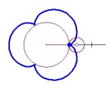
. The places where the cycles end are evenly spaced around the fixed circle and the locus has a cusp at these places.

What if we use other rational numbers? All of a sudden things are very different:

R=S=\tfrac{2}{3}\text{, }0\le t\le 2\pi

Now the circumference of the larger circle is not a multiple of the circumference of the smaller. To return the circle to its starting orientation we have to go around once more by letting t go from 0 to 4\pi . The first time around (from 0 to 2\pi ) is shown in orange and the rest of the path in blue.

R=S=\tfrac{2}{3},\quad 0\le t\le 4\pi

Investigation 1: Using the ratio of the radius of the fixed circle to the moving circle, determine how many times the moving circle must go around the fixed circle to draw a complete curve.
 

If  R=\frac{n}{d} is a rational number (reduced), then by increasing the maximum value of t to 2n\pi  the moving circle will return to its original position after n revolutions and after  that the curve will be retraced. This is the same regardless of whether \tfrac{n}{d} is greater than or less than 1.

We now turn our attention to the cusps; the places where the point “bounces off” the fixed circle.

Investigation 2: Using the ratio of the radius of the fixed circle to the moving circle, determine how many cusps the graph will have. 

For these curves, If R=\frac{n}{d} there are d places where the locus “bounces” of the fixed circle. These appear as cusps of the locus.

R=S=\tfrac{7}{5}\text{, }0\le t\le 14\pi

Finally, if R is not rational, the moving circle will never return to its original orientation and the locus will keep adding cusps as the circle continues to roll round the fixed circle

R=S=\sqrt{2},\quad 0\le t\le 100

Curves of this type, with the moving circle smaller or larger than the fixed circle and R = S, are called epicycloids. Epicycloids are a special case of Epitrochoids which will be the subject of the next post in this series.

Investigation 3: Determine the value of t for each cusp, of a graph with d cusps.  

Solution left as an exercise.

Investigation 4: Investigate the derivative at a cusp. 

Solution left as an exercise. This will be discussed in a later post.

References:

Cardioids: http://en.wikipedia.org/wiki/Cardioid

Epicycloids: http://en.wikipedia.org/wiki/Epicycloid

Epitrochoids: http://en.wikipedia.org/wiki/Epitrochoid

Corrections made July 5, 2014

Rolling Circles

A few weeks ago I covered some trigonometry classes for another teacher. They were studying polar and parametric graphs and the common curves limaçon, rose curves, cardioids, etc. I got to thinking about these curves. the next few posts will discuss what I learned. To help me see what was happening I made a Winplot animation. My “Roulette Generator” (RG) is a rather simple setup and turned out to be very well suited to study a variety of curves: cardioids, epicycloids, epitrochoids, hypochoids, and hypotrochoids to name a few. They are all examples of roulettes – curves generated by a point on a curve as it moves around anther curve. I considered only cases where both curves are circles. Calculus will make it appearance after the first few posts in this series. I hope you will find information here that will let you make a good project or investigation for calculus or precalculus students. The RG can be set to graph any number of situations as I will discuss. So here goes.


Roulettes – 1: Equations and the Roulette Generator.

In this post I will discuss the derivation of the parametric equations used to make the animations and some notes on how to use the RG. Later posts will discuss some of the various curves that result. I began with a simple cardioid.

R1

Cardioid R = S = 1

A cardioid is defined as the locus of a point on a circle as it rolls without slipping around another circle with the same radius. 

The setup described here will allow us to change the equations using sliders, for this and a number of related curves. The two circles with the same radii are shown in the figure below. The circle with center at C rolls counterclockwise around the circle with center at the origin, O. The point D traces the cardioid. The blue curve from F to D is the beginning of the cardioid. Cardioid setup pix The equations of the circles are: The circle centered at the origin with radius 1:

x\left( t \right)=\cos \left( t \right)\text{ and }y\left( t \right)=\sin \left( t \right)

The moving circle with center at C and radius R:

x\left( t \right)=(1+R)\cos (t)+R\cos (t) and

y\left( t \right)=(1+R)\sin \left( t \right)+R\sin \left( t \right).

The equation of the locus: In the figure above, the locus of the point marked D, as the moving circle rolls counterclockwise around the fixed circle, will be the path of the curves. A small portion of the curve is shown in blue running from F to D. In our investigations we will eventually want to place the moving point inside, on, or outside the moving circle. To do this we will use S as the distance from the center of the moving circle to the point we are watching. For the moment and for the simple cardioid, we will assume they are the same: R=S=1.

The ratio of the radius of the fixed circle to the radius of the moving circle is 1/R,  and will be of interest. The ratio can be adjusted by changing R. We can, therefore, keep the fixed circle’s radius constant and equal to one.

We will use vectors to write the locus. Before writing the individual vectors consider first that the arc length on both circles is always the same for all the curves and combinations of their radii:

\text{arc }EF=t=\text{arc }DE=R\left( \measuredangle DCE \right).

Therefore, \measuredangle DCE=\tfrac{1}{R}t. Then  \measuredangle BCD=\tfrac{\pi }{2}-\left( \tfrac{1}{R}t+t \right) Then the locus of D has the vector equation:

\overrightarrow{OD}=\overrightarrow{OA}+\overrightarrow{AC}+\overrightarrow{CB}+\overrightarrow{BD}

\overrightarrow{OD}=\left\langle (1+R)\cos (t),0 \right\rangle +\left\langle 0,\left( 1+R \right)\sin \left( t \right) \right\rangle +

\left\langle -S\sin \left( \tfrac{\pi }{2}-(\tfrac{1}{R}t+t) \right),0 \right\rangle +\left\langle 0,-S\cos \left( \tfrac{\pi }{2}-(\tfrac{1}{R}t+t) \right) \right\rangle

Notice that \left( \tfrac{1}{R}t+t \right) is the complement of \left( \tfrac{\pi }{2}-\left( \tfrac{1}{R}t+t \right) \right), so that \sin \left( \tfrac{\pi }{2}-(\tfrac{1}{R}t+t) \right)=\cos \left( \tfrac{1}{R}t+t \right) and  \cos \left( \tfrac{\pi }{2}-(\tfrac{1}{R}t+t) \right)=\sin \left( \tfrac{1}{R}t+t \right). The parametric equations of the path are

x\left( t \right)=(1+R)\cos \left( t \right)-S\cos \left( \tfrac{1}{R}t+t \right)

y\left( t \right)=\left( 1+R \right)\sin \left( t \right)-S\sin \left( \tfrac{1}{R}t+t \right)

You may enter these equations on any graphing calculator by entering specific values of R and S. You will have to re-type them for each different curve. With the RG you can make the changes easily with sliders.

The roulette generators: I used Winplot a free graphing program I’ve used for years. Here are the links so you can download Winplot or Winplot for Macs. the Winplot file containing the generator is here: Winplot Roulette Generator. [Sorry, this is no longer available here and WordPress will not accept Winplot files for download. Please contact me at lnmcmullin@aol.com and I’ll send you a copy.] The Winplot equations are discussed here: Notes on the Roulette Generator.

A Geometer’s Sketchpad version may be downloaded Geometer’s Sketchpad Roulette Generator. You will need Geometer’s Sketchpad to run this on a computer or the “Sketch Explorer” app for iPads and other tablets. A big ‘Thanks” to Audrey Weeks who was kind enough to make this for us. Audrey is the author of the Algebra in Motion and Calculus in Motion software. Audrey is my “go to” person when I have math questions.

Other graphers with sliders such as Geogebra and TI-Nspire will probably work as well. For those who wish to adapt this to some other graphing program there are some syntax consideration to making the one circle roll around the other and showing the path as the circle rolls. If you make your own generator on one of these other platforms, please send it along and I’ll post it and give you credit.

Experiment with the R and S sliders. In the next several posts well will do this and learn about various other curves.

Next: Epicycloids

References:

Cardioids: http://en.wikipedia.org/wiki/Cardioid

Roulettes: http://en.wikipedia.org/wiki/Roulette_(curve)

Algebra in Motion

Calculus in Motion