Hypocycloids and Hypotrochoids

Roulettes – 4: Hypocycloids and Hypotrochoids

In our last few posts we investigated rouletts, the curves that are formed by the locus of points attached to a circle as it rolls around the outside of a fixed circle. Depending on the ratio of the radii (and therefore the circumferences) of the circles these curves are the cardiods (equal radii), epicycloids (moving circle’s radius is less than the fixed circle), and epitrochoids (the point is in the interior or exterior of the moving circle).

In the first post of this series Roulette Generators are explained. Here are the files for Winplot or Geometer’s Sketchpad. Use them to quickly see the graphs of these curves by adjusting one or two parameters.

The parametric equations of these curves are below. and S are parameters that are adjusted for each curve.

x\left( t \right)=(1+R)\cos \left( t \right)-S\cos \left( \tfrac{1}{R}t+t \right)

y\left( t \right)=\left( 1+R \right)\sin \left( t \right)-S\sin \left( \tfrac{1}{R}t+t \right)

We shall now consider the curves that result when the moving circle rolls around the inside of the fixed circle. These curves are called hypocycloids and hypotrochoids. To generate today’s curves make the radius, R, of the moving circle negative.

The first seems almost a special case. Let R =  – 0.5 and S = 0.5 (below left) and then let R = S = – 0.5 (below right). The results are segments, which as we shall see are actually degenerate ellipses.

R = S = - 0.5

R = S = – 0.5

R = - 0.5,  S = + 0.5

R = – 0.5, S = + 0.5

In the following I will keep S negative. This makes the starting point (t = 0) on the positive side of the x-axis. If S is positive the starting point is to the left of the origin. The resulting curves are the same shapes by oriented differently (rotated a quarter-turn).

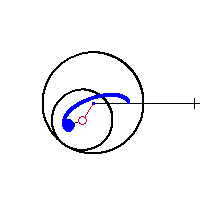
If R = – 1/2 the curves are ellipses. If S < R < 0 then ellipse stays inside the fixed circle (below left); if  R < S < 0 the ellipse extends outside the fixed circle (below right). If S = 0 the locus is a circle.

R = - 0.5,  S = - 0.3

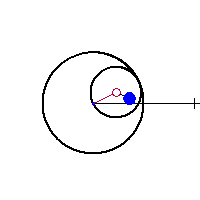
R = – 0.5, S = – 0.3

R = - 0.5,  S = - .75

R = – 0.5, S = – .75

Next we consider the more general case for which the moving circle’s radius is not exactly half of the fixed circle’s radius.

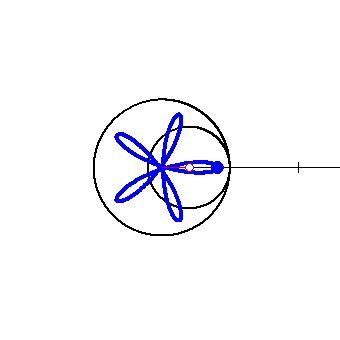
If R < S < 0, the point is in the interior of the moving circle and the graph is a series of loops (below left). When R = S , the point is on the circle, there is a star-like figure (below right). These are both called hypocycloids.

When S < R < 0 the point is outside the circle and the “stars” form rounded ends and get larger. These are the hypotrochoids (below center).

R = - 0.6,  S = - 0.3

R = – 0.6, S = – 0.3

R = S = - 0.6

R = S = – 0.6

R = - 0.6,  S = - 1

R = – 0.6, S = – 1

The next video shows the progression from S = 0 (a circle) to S = –2 and back again. (S is the distance between the center of the moving circle to the blue point.)

R = - 0.6, - 2 < S < 0,  A = 6pi

R = – 0.6, – 2 < S < 0, t = 6pi

Exploration 6: When R = –0.5 segments and ellipses are formed. Discuss how these are not really different from the cases with different negative values of R.
Exploration 7: In the case where R = S star-like figures are formed. The points of the “star” are cusps. Find the number and location of these cusps in terms of R. (Hint: see the discussion of the cusps in the second post in this series.)
Exploration 8: (Calculus) Find and discuss the derivative at the cusps when R = S.

This will be discussed in the next post. 

References:

Hyposycloid: http://en.wikipedia.org/wiki/Hypocycloid

Hypotrochoid: http://en.wikipedia.org/wiki/Hypotrochoid

Advertisement

Rolling Circles

A few weeks ago I covered some trigonometry classes for another teacher. They were studying polar and parametric graphs and the common curves limaçon, rose curves, cardioids, etc. I got to thinking about these curves. the next few posts will discuss what I learned. To help me see what was happening I made a Winplot animation. My “Roulette Generator” (RG) is a rather simple setup and turned out to be very well suited to study a variety of curves: cardioids, epicycloids, epitrochoids, hypochoids, and hypotrochoids to name a few. They are all examples of roulettes – curves generated by a point on a curve as it moves around anther curve. I considered only cases where both curves are circles. Calculus will make it appearance after the first few posts in this series. I hope you will find information here that will let you make a good project or investigation for calculus or precalculus students. The RG can be set to graph any number of situations as I will discuss. So here goes.


Roulettes – 1: Equations and the Roulette Generator.

In this post I will discuss the derivation of the parametric equations used to make the animations and some notes on how to use the RG. Later posts will discuss some of the various curves that result. I began with a simple cardioid.

R1

Cardioid R = S = 1

A cardioid is defined as the locus of a point on a circle as it rolls without slipping around another circle with the same radius. 

The setup described here will allow us to change the equations using sliders, for this and a number of related curves. The two circles with the same radii are shown in the figure below. The circle with center at C rolls counterclockwise around the circle with center at the origin, O. The point D traces the cardioid. The blue curve from F to D is the beginning of the cardioid. Cardioid setup pix The equations of the circles are: The circle centered at the origin with radius 1:

x\left( t \right)=\cos \left( t \right)\text{ and }y\left( t \right)=\sin \left( t \right)

The moving circle with center at C and radius R:

x\left( t \right)=(1+R)\cos (t)+R\cos (t) and

y\left( t \right)=(1+R)\sin \left( t \right)+R\sin \left( t \right).

The equation of the locus: In the figure above, the locus of the point marked D, as the moving circle rolls counterclockwise around the fixed circle, will be the path of the curves. A small portion of the curve is shown in blue running from F to D. In our investigations we will eventually want to place the moving point inside, on, or outside the moving circle. To do this we will use S as the distance from the center of the moving circle to the point we are watching. For the moment and for the simple cardioid, we will assume they are the same: R=S=1.

The ratio of the radius of the fixed circle to the radius of the moving circle is 1/R,  and will be of interest. The ratio can be adjusted by changing R. We can, therefore, keep the fixed circle’s radius constant and equal to one.

We will use vectors to write the locus. Before writing the individual vectors consider first that the arc length on both circles is always the same for all the curves and combinations of their radii:

\text{arc }EF=t=\text{arc }DE=R\left( \measuredangle DCE \right).

Therefore, \measuredangle DCE=\tfrac{1}{R}t. Then  \measuredangle BCD=\tfrac{\pi }{2}-\left( \tfrac{1}{R}t+t \right) Then the locus of D has the vector equation:

\overrightarrow{OD}=\overrightarrow{OA}+\overrightarrow{AC}+\overrightarrow{CB}+\overrightarrow{BD}

\overrightarrow{OD}=\left\langle (1+R)\cos (t),0 \right\rangle +\left\langle 0,\left( 1+R \right)\sin \left( t \right) \right\rangle +

\left\langle -S\sin \left( \tfrac{\pi }{2}-(\tfrac{1}{R}t+t) \right),0 \right\rangle +\left\langle 0,-S\cos \left( \tfrac{\pi }{2}-(\tfrac{1}{R}t+t) \right) \right\rangle

Notice that \left( \tfrac{1}{R}t+t \right) is the complement of \left( \tfrac{\pi }{2}-\left( \tfrac{1}{R}t+t \right) \right), so that \sin \left( \tfrac{\pi }{2}-(\tfrac{1}{R}t+t) \right)=\cos \left( \tfrac{1}{R}t+t \right) and  \cos \left( \tfrac{\pi }{2}-(\tfrac{1}{R}t+t) \right)=\sin \left( \tfrac{1}{R}t+t \right). The parametric equations of the path are

x\left( t \right)=(1+R)\cos \left( t \right)-S\cos \left( \tfrac{1}{R}t+t \right)

y\left( t \right)=\left( 1+R \right)\sin \left( t \right)-S\sin \left( \tfrac{1}{R}t+t \right)

You may enter these equations on any graphing calculator by entering specific values of R and S. You will have to re-type them for each different curve. With the RG you can make the changes easily with sliders.

The roulette generators: I used Winplot a free graphing program I’ve used for years. Here are the links so you can download Winplot or Winplot for Macs. the Winplot file containing the generator is here: Winplot Roulette Generator. [Sorry, this is no longer available here and WordPress will not accept Winplot files for download. Please contact me at lnmcmullin@aol.com and I’ll send you a copy.] The Winplot equations are discussed here: Notes on the Roulette Generator.

A Geometer’s Sketchpad version may be downloaded Geometer’s Sketchpad Roulette Generator. You will need Geometer’s Sketchpad to run this on a computer or the “Sketch Explorer” app for iPads and other tablets. A big ‘Thanks” to Audrey Weeks who was kind enough to make this for us. Audrey is the author of the Algebra in Motion and Calculus in Motion software. Audrey is my “go to” person when I have math questions.

Other graphers with sliders such as Geogebra and TI-Nspire will probably work as well. For those who wish to adapt this to some other graphing program there are some syntax consideration to making the one circle roll around the other and showing the path as the circle rolls. If you make your own generator on one of these other platforms, please send it along and I’ll post it and give you credit.

Experiment with the R and S sliders. In the next several posts well will do this and learn about various other curves.

Next: Epicycloids

References:

Cardioids: http://en.wikipedia.org/wiki/Cardioid

Roulettes: http://en.wikipedia.org/wiki/Roulette_(curve)

Algebra in Motion

Calculus in Motion