Roulettes – 5: Calculus Considerations.
In the first post of this series Roulette Generators (RG) are explained. Here are the files for Winplot or Geometer’s Sketchpad. Use them to quickly see the graphs of these curves by adjusting one or two parameters.
While writing this series of posts I was intrigued by the cusps that appear in some of the curves. In Cartesian coordinates you think of a cusp as a place where the curves is continuous, but the derivative is undefined, and the tangent line is vertical. Cusps on the curves we have been considering are different.
The equations of the curves formed by a point attached to a circle rolling around a fixed circle in the form we have been using are:


For example, let’s consider the case with 
Epicycloid with R = S = 1/3
The equations become

The derivative is

The cusps are evenly spaced one-third of the way around the circle and appear at  . At the cusps dy/dx is an indeterminate form of the type 0/0. (Note that at
  ,
,  and likewise for the sine.) Since derivatives are limits, we can apply L’Hôpital’s Rule and find that at

This is, I hope, exactly what we should expect. As the curve enters and leaves the cusp it is tangent to the line from the cusp to the origin. (The same thing happens at the other two cusps.) At the cusps the moving circle has completed a full revolution and thus, the line from its center to the center of the fixed circle goes through the cusp and has a slope of tan(t).
The cusps will appear where the same t makes dy/dt = 0 and dx/dt =0 simultaneously.
The parametric derivative is defined at the cusp and is the slope of the line from the cusp to the origin. Now I may get an argument on that, but that’s the way it seems to me.
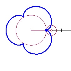
A look at the graph of the derivative in parametric form may help us to see what is going on. In the next figure with the graph of the curve is in blue. The velocity vector is shown twice (arrows). The first is attached to the moving point and shows the direction and its length shows the speed of the movement. The second shows the velocity vector as a position vector (tail at the origin). The orange graph is the path of the velocity vector’s tip – the parametric graph of the velocity. Note that these vectors are the same (i.e. they have the same direction and magnitude)
The video shows the curve moving through the cusp at. Notice that as the graph passes through the cusp the velocity vector changes from pointing down to the right, to the zero vector, to pointing up to the left. The change is continuous and smooth.
Velocity near a cusp.
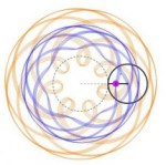
Here is the whole curve being drawn with its velocity and the velocity vectors.
Epicycloid with velocity vectors
(If you are using the Winplot file you graph the velocity this way. Open the inventory with CTRL+I, scroll down to the bottom and select, one at a time, the last three lines marked “hidden”, and then click on “Graph.”). The Geometer’s Sketchpad version has a button to show the derivative’s graph and the velocity vectors.
The general equation of the derivative (velocity vector) is


Notice that the derivative has to same form as a roulette.
Finally, I have to mention how much seeing the graphs in motion have helped me understand, not just the derivatives, but all of the curves in this series and the ones to come. To experiment, to ask “what if … ?” questions, and just to play is what technology should be used for in the classroom. See what your students can find using the RGs.
Exploration and Challenge:
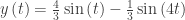
Consider the epitrochoid  .
.
- Find its derivative as a parametric equation and graph it with a graphing program or calculator. (Straight forward)
- Are the graph of the derivative and the graph of the rose curve given in polar form by
 the same? Justify your answer. (Warning: The graphs certainly look the same. I have not been able to do show they are the same (which certainly doesn’t prove anything), so they may not be the same.) Please post your answer using the “Leave a Reply” box at the end of this post.
Next: Roulette Art.

θ
θ
to convert from polar to parametric form,
and
(Hint: use the product rule on the equations in the previous bullet).
(motion towards or away from the pole),
(motion in the vertical direction) or
.


 changes sign.
 . The integral is the difference between whatever f represents at b and what it represents at a. (2009 AB 2 c, AB 3c, 2013 AB3/BC3 c)
 for
for  . Find the location of the minimum value of f(x). Justify your answer three different ways (without reference to each other).
 from the first. (From the previous posts: if
  then there are d dips, loops, or cusps in n full revolutions). Both graphs will have the same R value.


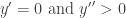
 , R = 0.00667 and slightly less than a full revolution. Make the image size (under the file tab) 12.3 x 12.3 (the units are cm.), or 465 x 465 pixels (type @ after the number to use pixels). Amazing!
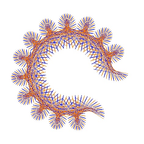


 there will be cusps, if
  dips, and if
  loops. (Of course, you could have your students discover this on their own.) Experiment with this to make other designs.


