
Good Question 11 – or not. 
The question below appears in the 2016 Course and Exam Description (CED) for AP Calculus (CED, p. 54), and has caused some questions since it is not something included in most textbooks and has not appeared on recent exams. The question gives a Riemann sum and asks for the definite integral that is its limit. Another example appears in the 2016 “Practice Exam” available at your audit website; see question AB 30. This type of question asks the student to relate a definite integral to the limit of its Riemann sum. These are called reversal questions since you must work in reverse of the usual order. Since this type of question appears in both the CED examples and the practice exam, the chances of it appearing on future exams look good.
To the best of my recollection the last time a question of this type appeared on the AP Calculus exams was in 1997, when only about 7% of the students taking the exam got it correct. Considering that by random guessing about 20% should have gotten it correct, this was a difficult question. This question, the “radical 50” question, is at the end of this post.
Example 1
Which of the following integral expressions is equal to
?
There were 4 answer choices that we will consider in a minute.
The first key to answering the question is to recognize the limit as a Riemann sum. In general, a right-side Riemann sum for the function f on the interval [a, b] with n equal subdivisions, has the form:

To evaluate the limit and express it as an integral, we must identify, a, b, and f. I usually begin by looking for 

Usually, you can start by considering a = 0 , which means that the 


The answer choices are
(A) 


The correct choice is (A), but notice that choices B, C, and D can be eliminated as soon as we determine that b = a + 1. That is not always the case.
Let’s consider another example:
Example 2:

As before consider 


BUT
What if we take a = 2? If so, the limit is 
And now one of the “problems” with this kind of question appears: the answer written as a definite integral is not unique!
Not only are there two answers, but there are many more possible answers. These two answers are horizontal translations of each other, and many other translations are possible, such as 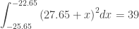
The same thing can occur in other ways. Returning to example 1,and using something like a u-substitution, we can rewrite the original limit as 
Now b = a + 3 and the limit could be either 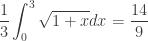

My opinions about this kind of question.
The real problem with the answer choices to Example 1 is that they force the student to do the question in a way that gets one of the answers. It is perfectly reasonable for the student to approach the problem a different way, and get a different correct answer that is not among the choices. This is not good.
The problem could be fixed by giving the answer choices as numbers. These are the numerical values of the 4 choices:(A) 14/9 (B) 14/3 (C) 14/3 (D) 
A related problem is this: The limit of a Riemann sum is a number; a definite integral is a number. Therefore, any definite integral, even one totally unrelated to the Riemann sum, which has the correct numerical value, is a correct answer.
I’m not sure if this type of question has any practical or real-world use. Certainly, setting up a Riemann sum is important and necessary to solve a variety of problems. After all, behind every definite integral there is a Riemann sum. But starting with a Riemann sum and finding the function and interval does not seem to me to be of practical use.
The CED references this question to MPAC 1: Reasoning with definitions and theorems, and to MPAC 5: Building notational fluency. They are appropriate,and the questions do make students unpack the notation.
My opinions notwithstanding, it appears that future exams will include questions like these.
These questions are easy enough to make up. You will probably have your students write Riemann sums with a small value of n when you are teaching Riemann sums leading up to the Fundamental Theorem of Calculus. You can make up problems like these by stopping after you get to the limit, giving your students just the limit, and having them work backwards to identify the function(s) and interval(s). You could also give them an integral and ask for the associated Riemann sum. Question writers call questions like these reversal questions since the work is done in reverse of the usual way.
Here is the question from 1997, for you to try. The answer is below.

Answer B. Hint n = 50
Revised 5-5-2022
 by the tabular method (See

 . Example 2 shows why you want (need) to stop. In Example 1 you will have


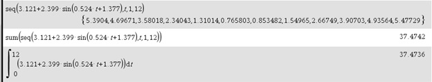
 , where R is measured in inches and t is the time in months, t = 1 being January. Use integration to approximate the normal annual rainfall. Hint: Integrate over the interval [0,12].
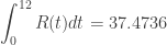 inches. You could quit here and go on to the next question, but …
 is not.
 .
.
 . For example the amount of rain that falls in June is given by
 .
. . So the sine function takes on (almost) all its values in a year, as you would expect. Since the sine values all but cancel each other out
 . Close!
 this must be close to the average rainfall each month. The average rainfall is
  inches. Close, again!
 dollars per meter. Profit was defined as the difference between the money the company received for selling the cable minus the cost of producing the cable.


 in the context of the problem. Since the answer is probably not immediately obvious, here is the reasoning involved.
 .
. , and therefore,
  by the Fundamental Theorem of Calculus (FTC).
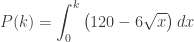


 when x = 400 and P(400)= $16,000.
 and for
 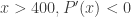 therefore, the maximum profit occurs at x = 400. (The First Derivative Test).
 Another of my favorite questions from past AP exams is from 2000 question AB 4. If memory serves it is the first of what became known as an “In-out” question. An “In-out” question has two rates that are working in opposite ways, one filling a tank and the other draining it.
 always has a solution of the form
 .
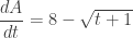
. gives the net amount of change over the interval of integration
 ![[{{t}_{0}},t]](https://s0.wp.com/latex.php?latex=%5B%7B%7Bt%7D_%7B0%7D%7D%2Ct%5D&bg=ffffff&fg=333333&s=0&c=20201002) . When this is added to the initial amount the result is an expression that gives the amount at any time t.
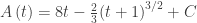
. When this is added to the initial amount the result is an expression that gives the amount at any time t.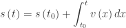 where
where 
 gallons per minute.

 since nothing has leaked out yet, so C = -2/3
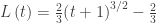


 or
or .
.
 , so
, so 

 minutes the amount of water in the tank was a maximum and to justify their answer. The usual method is to find the derivative of the amount, A(t), set it equal to zero, and then solve for the time.
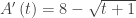
 when t = 63
 . After finding that t = 63, the answer may be justified by stating that before this time more water is being pumped in than is leaking out and after this time the rate at which water leaks out is greater than the rate at which it is pumped in, so the maximum must occur at t = 63.
