Another in my occasional series on Good Questions to teach from. This is the Mighty Cable Company question from the 2009 AB Calculus exam, number 3
This question presented students with a different situation than had been seen before. It is a pretty standard “in-out” question, except that what was going in and out was money. Students were told that the Mighty Cable Company sold its cable for $120 per meter. They were also told that the cost of the cable varied with its distance from the starting end of the cable. Specifically, the cost of producing a portion of the cable x meters from the end is  dollars per meter. Profit was defined as the difference between the money the company received for selling the cable minus the cost of producing the cable.
Students had a great deal of trouble answering this question. (The mean was 1.92 out of a possible 9 points. Fully, 36.9% of students earned no point; only 0.02% earned all 9 points.) This was probably because they had difficulty in interpreting the question and translating it into the proper mathematical terms and symbols. Since economic problems are not often seen on AP Calculus exams, students needed to be able to use the clues in the stem:
- The $120 per meter is a rate. This should be deduced from the units: dollars per meter.
- The cost of producing the portion of cable x meters from one end cable is also a rate for the same reason. In economics this is called the marginal cost; the students did not need to know this term.
- The profit is an amount that is a function of x, the length of the cable.
Part (a): Students were required to find the profit from the sale of a 25-meter cable. This is an amount. As always, when asked for an amount, integrate a rate. In this case integrate the difference between the rate at which the cable sells and the cost of producing it.

or

Part (b): Students were asked to explain the meaning of  in the context of the problem. Since the answer is probably not immediately obvious, here is the reasoning involved.
This is the integral of a rate and therefore, gives the amount (of money) needed to manufacture the cable. This can be found by a unit analysis of the integrand:  .
.
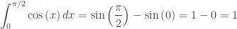
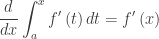
Let C be the cost of production, so  , and therefore,
  by the Fundamental Theorem of Calculus (FTC).
Therefore, is the difference in dollars between the cost of producing a cable 30 meters long, C(30), and the cost of producing a cable 25 meters long, C(25). (Another acceptable is that the integral is the cost in dollars of producing the last 5 meters of a 30 meter cable.)
Part (c): Students were asked to write an expression involving an integral that represents the profit on the sale of a cable k meters long.
Part (a) serves as a hint for this part of the question. Here the students should write the same expression as they wrote in (a) with the 25 replaced by k.
or

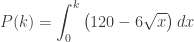
Part d: Students were required to find the maximum profit that can be earned by the sale of one cable and to justify their answer. Here they need to find when the rate of change of the profit (the marginal profit) changes from positive to negative.
Using the FTC to differentiate either of the answers in part (c) or by starting fresh from the given information:

 when x = 400 and P(400)= $16,000.
Justification: The maximum profit on the sale of one cable is $16,000 for a cable 400 meters long. For  and for
  therefore, the maximum profit occurs at x = 400. (The First Derivative Test).
Once students are familiar with in-out questions, this is a good question to challenge them with. The actual calculus is not that difficult or unusual but concentrating on the translation of the unfamiliar context into symbols and calculus ideas is different. Show them how to read the hints in the problem such as the units.
Steel cable or steel wire rope as it is called also has some interesting geometry in its construction. You can find many good illustrations of this, such as the ones below, by Googling “steel wire rope.”
This slideshow requires JavaScript.


 is a partition of that interval, and
 ![x_{i}^{*}\in [{{x}_{{i-1}}},{{x}_{i}}]](https://s0.wp.com/latex.php?latex=x_%7Bi%7D%5E%7B%2A%7D%5Cin+%5B%7B%7Bx%7D_%7B%7Bi-1%7D%7D%7D%2C%7B%7Bx%7D_%7Bi%7D%7D%5D&bg=ffffff&fg=333333&s=0&c=20201002) , then
, then
 is called the “norm of the partition” and is the longest subinterval in the partition. Usually, all the subintervals are the same length,
  , and this is the last you will hear of the norm. With all the subdivisions of the same length this can be written as
 .
.
 , to be the number in each subinterval guaranteed by the MVT for that subinterval.
 . Making this substitution, we have


 and
and  ,
, .
. .
. . With a little help they should arrive at
 .
. .
. .
.
 ?
?
 ,
,
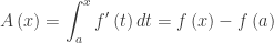
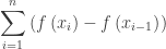
 to
to  . What is the net change in f over this interval? Easy it’s
  . No problem, but way too easy for a calculus class. So let’s try a harder way!
 .
. .
. part. What to do?
 or
or  .
.
 .
. .
. .
. on the interval [1, 4]. Hover and click on the figure below.
