When are we ever …?

Allen Wohlmer

The following answer to a question we’ve all been asked was posted yesterday on a private Facebook page for AP Calculus readers. The author, Allen Wolmer is a teacher and AP Calculus reader. He teaches at Yeshiva Atlanta High School, in Atlanta, Georgia. I reprint it here with his kind permission.

Thank you, Allen.


A colleague of mine teaching high school math asked me the following:

“So some of my kids are struggling with the math concepts and ideas (why do I need to learn this? When will I ever use factoring/polynomials?). I would say most of my students have not had a particularly good relationship with math in the past.

I have answered these questions, with responses like financial jobs, accounting, econ, but they have no interest in these types of jobs/real world applications.

I have also talked about logic, problem solving, and puzzles.
Do you have any advice for me, and or ideas to share with them?”

Here is my reply:

“Glad to help.
First of all, recognize that, for the most part, the kids aren’t really interested in your answer. They are just being lazy and looking for a reason, any reason, to not do work, any work.
Now, how do you answer? Well, you can try the face value approach, that is describing engineering, actuary, etc., but that will be meaningful to just a handful of students, and they’re not the ones asking the question anyway.

So, I turn it around. I ask the boys how many go the gym or health club or weight room to work out. Hands quickly shoot up (after all, they want to be cool in front of their buds and the chicks). I then ask them how many use the pec machine (it’s the one where you raise your arms to shoulder level and bring the elbows together). I demonstrate with the motion. Many of them admit they use the machine. I then ask them when they would ever use that motion in real life. The answer, of course, is NEVER! So, why do you do it, I ask them. I answer for them “because it strengthens your muscles!”

And that’s why we study mathematics: to strengthen our mental muscles. We’re not really studying math, I tell them. We’re studying how to analyze and understand problems when we read them. What do we know? What do we not know? What are we trying to find?

We’re learning how to pay attention to detail. We’re learning how to be precise in our thinking and our work. We’re learning how to be neat in our work. We’re learning to look for patterns. We’re learning to look for similarities to other problems we have solved. We’re learning how to look at our results and determine if they make sense or not.
In other words, we’re learning how to think critically and solve problems. We’re doing it in the context of learning mathematics, but that’s only because that’s the best environment to do it in.

Then I tell them never to ask that #$%^%$# question again and to shut the #$%^&*&^% up and get back to work!

Sincerely,
Allen Wolmer”

.

Advertisement

Determining the Indeterminate 2

The other day someone asked me a question about the implicit relation {{x}^{3}}-{{y}^{2}}+{{x}^{2}}=0. They had been asked to find where the tangent line to this relation is vertical. They began by finding the derivative using implicit differentiation:

3{{x}^{2}}-2y\frac{dy}{dx}+2x=0

\displaystyle \frac{dy}{dx}=\frac{3{{x}^{2}}+2x}{2y}

The derivative will be undefined when its denominator is zero. Substituting y = 0 this into the original equation gives {{x}^{3}}-0+{{x}^{2}}=0. This is true when x = –1 or when x = 0. They reasoned that there will be a vertical tangent when x = –1 (correct) and when x = 0 (not so much). They quite wisely looked at the graph.

relation 1

{{x}^{3}}-{{y}^{2}}+{{x}^{2}}=0

The graph appears to run from the first quadrant, through the origin into the third quadrant, up to the second quadrant with a vertical tangent at x = –1, and then through the origin again and down into the fourth quadrant. It looks like a string looped over itself.

What’s going on at the origin? Where is the vertical tangent at the origin?

The short answer is that vertical tangents occur when the denominator of the derivative is zero and the numerator is not zero.  When x = 0 and y = 0 the derivative is an indeterminate form 0/0.

In this kind of situation an indeterminate form does not mean that the expression is infinite, rather it means that some other way must be used to find its value. L’Hôpital’s Rule comes to mind, but the expression you get results in another 0/0 form and is no help (try it!).

My thought was to solve for y and see if that helps:

y=\pm \sqrt{{{x}^{3}}+{{x}^{2}}}

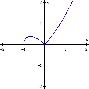
The graph consists of two parts symmetric to the x-axis, in the same way a circle consists of two symmetric parts above and below the x-axis. The figure below shows the top half.

y=+\sqrt{{{x}^{3}}+{{x}^{2}}}

So, the graph does not run from the first quadrant to the third; rather, at the origin it “bounces” up into the second quadrant. The lower half is congruent and is the reflection of this graph in the x-axis.

So, what happens at the origin and why?

The derivative of the top half is \displaystyle \frac{dy}{dx}=\frac{3{{x}^{2}}+2x}{2\sqrt{{{x}^{3}}+{{x}^{2}}}}. Notice that this is the same as the implicit derivative above. Now a little simplifying; okay a lot of simplifying – who says simplifying isn’t that big a deal?

\displaystyle \frac{dy}{dx}=\frac{x\left( 3x+2 \right)}{2\sqrt{{{x}^{2}}\left( x+1 \right)}}=\frac{x\left( 3x+2 \right)}{2\left| x \right|\sqrt{x+1}}=\left\{ \begin{matrix} \frac{3x+2}{2\sqrt{x+1}} & x>0 \\ -\frac{3x+2}{2\sqrt{x+1}} & x<0 \\ \end{matrix} \right.

Now we see what’s happening. As x approaches zero from the right, the derivative approaches +1, and as x approaches zero from the left, the derivative approaches –1.  This agrees with the graph. Since the derivative approaches different values from each side, the derivative does not exist at the origin – this is not the same as being infinite.  (For the lower half, the signs of the derivative are reversed, due to the opposite sign of the denominator.)

The tangent lines at the origin are x = 1 on the right, and x = –1 on the left, hardly vertical.

What have we learned?

  1. Indeterminate forms do not necessarily indicate an infinite value. An indeterminate form must be investigated further to see what you can learn about a function, relation, or graph.
  2. Sometimes simplifying, or at least changing the form of an expression, is helpful and therefore necessary.

Extension: Using a graphing utility that allows sliders (Winplot, GeoGebra, Desmos, etc)  enter A{{x}^{3}}-B{{y}^{2}}+C{{x}^{2}}=0 and explore the effects of the parameters on the graph.

_________________________

The Man Who Tried to Redeem the World with Logic

WALTER PITTS (1923-1969): Walter Pitts’ life passed from homeless runaway, to MIT neuroscience pioneer, to withdrawn alcoholic. (Estate of Francis Bello / Science Source)

WALTER PITTS (1923-1969): Walter Pitts’ life passed from homeless runaway, to MIT neuroscience pioneer, to withdrawn alcoholic. (Estate of Francis Bello / Science Source)

I ran across this article that you might find interesting. It is about Walter Pitts one of the twentieth century’s most important mathematicians we, or at least I, have never heard of.  It is from the February 5, 2015 of the science magazine Nautilus


The Fundamental Theorem of Calculus

The Fundamental Theorem of Calculus or FTC, as its name suggests, is a very important idea. It is not sufficient to present the formula and show students how to use it. Show them where it comes from.

Here is an approach to demonstrate the FTC. I try to sneak up on the result by proposing a problem and then solving it. Here is the outline.

Suppose we have a differentiable function f that goes from \left( a,f\left( a \right) \right) to \left( b,f\left( b \right) \right). What is the net change in f over this interval? Easy it’s f\left( b \right)-f\left( a \right).  No problem, but way too easy for a calculus class. So let’s try a harder way!

Partition the interval [a, b] as you would for a Riemann sum, and calculate the change in f on each subinterval. The subintervals may be the same width or not. The change in y on the general subinterval [xi-1, xi] is f\left( {{x}_{i}} \right)-f\left( {{x}_{i-1}} \right).

Approximate the net change over the whole interval by adding these \displaystyle \sum\limits_{i=1}^{n}{\left( f\left( {{x}_{i}} \right)-f\left( {{x}_{i-1}} \right) \right)} .
Is this a Riemann sum? No it is not! There is no \Delta x part. What to do?

The expression f\left( {{x}_{i}} \right)-f\left( {{x}_{i-1}} \right) looks familiar.
It is part of the equation for the Mean Value Theorem: \displaystyle {f}'\left( c \right)=\frac{f\left( b \right)-f\left( a \right)}{b-a} or {f}'\left( c \right)\left( b-a \right)=f\left( b \right)-f\left( a \right).
If we adapt this to the subinterval letting ci be the number guaranteed by the MVT on each subinterval  [xi-1, xi], then f\left( {{x}_{i}} \right)-f\left( {{x}_{i-1}} \right)={f}'\left( {{c}_{i}} \right)\left( {{x}_{i}}-{{x}_{i-1}} \right)

We can rewrite the sum in step 3 as \displaystyle \sum\limits_{i=1}^{n}{\left( f\left( {{x}_{i}} \right)-f\left( {{x}_{i-1}} \right) \right)}=\sum\limits_{n=1}^{n}{\left( {f}'\left( {{c}_{i}} \right)\left( {{x}_{i}}-{{x}_{i-1}} \right) \right)} .

  1. This is a Riemann sum and therefore, \displaystyle \underset{n\to \infty }{\mathop{\lim }}\,\sum\limits_{n=1}^{n}{\left( {f}'\left( {{c}_{i}} \right)\left( {{x}_{i}}-{{x}_{i-1}} \right) \right)}=\int_{a}^{b}{{f}'\left( c \right)dx} .
  2. So what is this equal to? We have already found what this limit is in step 1, so we now have:

\displaystyle \int_{a}^{b}{{f}'\left( x \right)dx}=f\left( b \right)-f\left( a \right).

This is called the FTC. And it is important.

The first thing it tells us is that the integral of a rate of change is the (net) amount of change. This will help us do a variety of problems.

The second thing it tells us is that, if we can find a function of which the integrand is the derivative (i.e. its antiderivative), then we can find the value of a definite integral by evaluating an antiderivative at the endpoints and subtracting. No more struggling with trying to find the limit of Riemann sums or graphing the function and hoping you can break it into regions with easy to find areas. All we need is an antiderivative and then one quick computation will do the trick from now on.

There is more to the FTC. This will be the subject of the next post.

The Definition of the Definite Integral

From the last post, it seems pretty obvious that as the number of rectangles in a Riemann sum increases or, what amounts to the same thing, the width of the sub-intervals decreases, the Riemann sum approaches the area of the region between a graph and the x-axis. The figures below show left-Riemann sums for the function f\left( x \right)=1+{{x}^{2}} on the interval [1, 4]. Hover and click on the figure below.

This slideshow requires JavaScript.

As the number of rectangles increases, they fill up more and more of the region. The sums increase, yet, their sum is always less than the area. They form an increasing sequence which is bounded above and therefore approaches its least upper bound (the area) as a limit.

Right-side rectangles work almost the same way. The sums form a decreasing sequence that is bounded below by the area and thus they approach the same limit.

All of the other Riemann sums must be between these two (at least for this example) and thus all approach the same limit.

This limit is called the definite integral for f on the interval [a, b], denoted by the new symbol below.

\displaystyle \underset{n\to \infty }{\mathop{\lim }}\,\sum\limits_{i=1}^{n}{f\left( x_{i}^{*} \right)\left( {{x}_{i}}-{{x}_{i-1}} \right)}=\underset{\Delta x\to 0}{\mathop{\lim }}\,\sum\limits_{i=1}^{n}{f\left( x_{i}^{*} \right)\Delta x=\int_{a}^{b}{f\left( x \right)dx}}

The notation has the advantage of being simpler to write than all the limit stuff and it shows us the interval which the limits do not. (For now consider the dx as a stand-in for \Delta x.)

The disadvantage of the notation is that, as we use it for real applications, the concept of Riemann sums often gets lost. The integrals become formulas and they get memorized but not understood.

Remember: behind every (any, all) definite integral is a Riemann sum.  As we look at applications, we should always look for the Riemann sum and how it is set up. This will tell us what the definite integral should be. We will not need to be too fussy about the subscripts and such; in fact, we will almost ignore them, but we will look carefully at the Riemann sum rectangles.

Riemann Sums

In our last post we discussed what are called Riemann sums. A sum of the form \displaystyle \sum\limits_{i=1}^{n}{f\left( x_{i}^{*} \right)\left( {{x}_{i}}-{{x}_{i-1}} \right)} or the form \sum\limits_{i=1}^{n}{f\left( x_{i}^{*} \right)\Delta x} (with the meanings from the previous post) is called a Riemann sum.

The three most common are these and depend on where the x_{i}^{*} is chosen.

  • Left-Riemann sum, L, uses the left side of each sub-interval, so x_{i}^{*}={{x}_{n-1}}.
  • Right-Riemann sum, R, uses the right side of each sub-interval, so x_{i}^{*}={{x}_{i}}.
  • Midpoint-Riemann sum, M, uses the midpoint of each interval, so x_{i}^{*}=\tfrac{1}{2}\left( {{x}_{i-1}}+{{x}_{i}} \right).

For the AP Exams students should know these and be able to compute them. The actual values are often given in a table, so the long computation of the function values is not necessary.

Another way of approximating the area between the graph and the x-axis is to use trapezoids formed by joining the points at the ends of each sub-interval. The areas can be figured individually and added or the value, T, can be found by averaging the left- and right-Riemann sums, T=\tfrac{1}{2}\left( L+R \right). This trapezoid approximation is usually closer to the true value than the other left- or right sums.

Whenever you are dealing with approximations, you should have some sense of how good they are. All of the approximations discussed will get closer to the true area if more values (more partition points) are used.

If the graph is increasing on the interval, then the left-sum is an underestimate of the actual value and the right-sum is an overestimate.  If the curve is decreasing, then the right-sums are underestimates and the left-sums are overestimates. (To see why, draw a sketch.)

If the graph is concave up the trapezoid approximation is an overestimate, and the midpoint is an underestimate. If the graph is concave down, then trapezoids give an underestimate and the midpoint an overestimate. (To see how this works, draw a sketch. For the midpoint draw the tangent line at the midpoint to the sides of the sub-interval; this trapezoid has the same area as the rectangle drawn at the midpoint of the interval. Why?)

If the graphs are not monotone on the interval or change concavity, then all bets are off.

For all of the Riemann sums, including those not mentioned above, as the number of partition points increase (n\to \infty ), or the width of the all the sub-interval decrease (\Delta x\to 0), the limit of a Riemann sum approaches the area between the graph and the x-axis. This will be the subject of the next post.


Corrected 11-28-2017


Flying to Integrationland

Here is a problem similar to the one in the last post, but with foibles of its own.

The speed of an airplane in miles per hour is given at half-hour intervals in the table below. Approximately how far does the airplane travel in the three hours given in the table? How far is it from the airport?

Elapsed time (hours)   0 0.5 1 1.5 2 2.5 3
Speed  (miles per hour)    375    390    400    390    385    350    345

In addition to just finding the estimates, compare this situation with the Pump Problem from the last post. Some points to consider

    1. Answers between 1130 and 1145 miles are reasonable, if students proceed as they did with the Pump Problem. However, we cannot be sure since we do not know the speeds between the values recorded. In the Pump Problem we were told the pump was slowing down, so we could be sure the actual amount was between the values computed.
    2. Based on the information in the table what is the low and high estimates of the total distance? What assumptions do you make for these estimates? (Low = 1117.5 miles, high = 1157.5 miles assuming the plane flew at the slowest (fastest) speed in the table for the entirety of each 1/2-hour interval.)
    3. We also do not know where the plane started or which directions (plural) it was flying. So we have no way to tell how far it was from the airport (although we hope it gets to some airport eventually).
    4. What are the units? If we graph this as we did in the Pump Problem the various rectangles have dimensions of (miles/hour) by hours, so the “area” is miles (a linear unit).

Next: Jobs, Jobs, Jobs