Unit 5 covers the application of derivatives to the analysis of functions and graphs. Reasoning and justification of results are also important themes in this unit. (CED – 2019 p. 92 – 107). These topics account for about 15 – 18% of questions on the AB exam and 8 – 11% of the BC questions.
Reasoning and writing justification of results are mentioned and stressed in the introduction to the topic (p. 93) and for most of the individual topics. See Learning Objective FUN-A.4 “Justify conclusions about the behavior of a function based on the behavior of its derivatives,” and likewise in FUN-1.C for the Extreme value theorem, and FUN-4.E for implicitly defined functions. Be sure to include writing justifications as you go through this topic. Use past free-response questions as exercises and also as guide as to what constitutes a good justification. Links in the margins of the CED are also helpful and give hints on writing justifications and what is required to earn credit. See the presentation Writing on the AP Calculus Exams and its handout
Topics 5.1
Topic 5.1 Using the Mean Value Theorem While not specifically named in the CED, Rolle’s Theorem is a lemma for the Mean Value Theorem (MVT). The MVT states that for a function that is continuous on the closed interval and differentiable over the corresponding open interval, there is at least one place in the open interval where the average rate of change equals the instantaneous rate of change (derivative). This is a very important existence theorem that is used to prove other important ideas in calculus. Students often confuse the average rate of change, the mean value, and the average value of a function – See What’s a Mean Old Average Anyway?
Topics 5.2 – 5.9
Topic 5.2 Extreme Value Theorem, Global Verses Local Extrema, and Critical Points An existence theorem for continuous functions on closed intervals
Topic 5.3 Determining Intervals on Which a Function is Increasing or Decreasing Using the first derivative to determine where a function is increasing and decreasing.
Topic 5.4 Using the First Derivative Test to Determine Relative (Local) Extrema Using the first derivative to determine local extreme values of a function
Topic 5.5 Using the Candidates’ Test to Determine Absolute (Global) Extrema The Candidates’ test can be used to find all extreme values of a function on a closed interval
Topic 5.6 Determining Concavity of Functions on Their Domains FUN-4.A.4 defines (at least for AP Calculus) When a function is concave up and down based on the behavior of the first derivative. (Some textbooks may use different equivalent definitions.) Points of inflection are also included under this topic.
Topic 5.7 Using the Second Derivative Test to Determine Extrema Using the Second Derivative Test to determine if a critical point is a maximum or minimum point. If a continuous function has only one critical point on an interval, then it is the absolute (global) maximum or minimum for the function on that interval.
Topic 5.8 Sketching Graphs of Functions and Their Derivatives. First and second derivatives give graphical and numerical information about a function and can be used to locate important points on the graph of the function.
Topic 5.9 Connecting a Function, Its First Derivative, and Its Second Derivative. First and second derivatives give graphical and numerical information about a function and can be used to locate important points on the graph of the function.
Topics 5.10 – 5.11
Optimization is important application of derivatives. Optimization problems as presented in most text books, begin with writing the model or equation that describes the situation to be optimized. This proves difficult for students, and is not “calculus” per se. Therefore, writing the equation has not be asked on AP exams in recent years (since 1983). Questions give the expression to be optimized and students do the “calculus” to find the maximum or minimum values. To save time, my suggestion is to not spend too much time writing the equations; rather concentrate on finding the extreme values.
Topic 5.10 Introduction to Optimization Problems
Topic 5.11 Solving Optimization Problems
Topics 5.12
Topic 5.12 Exploring Behaviors of Implicit Relations Critical points of implicitly defined relations can be found using the technique of implicit differentiation. This is an AB and BC topic. For BC students the techniques are applied later to parametric and vector functions.
Timing
Topic 5.1 is important and may take more than one day. Topics 5.2 – 5.9 flow together and for graphing they are used together; after presenting topics 5.2 – 5.7 spend the time in topics 5.8 and 5.9 spiraling and connecting the previous topics. Topics 5.10 and 5.11 – see note above and spend minimum time here. Topic 5.12 may take 2 days.
The suggested time for Unit 5 is 15 – 16 classes for AB and 10 – 11 for BC of 40 – 50-minute class periods, this includes time for testing etc.
Finally, were I still teaching, I would teach this unit before Unit 4. The linear motion topic (in Unit 4) are a special case of the graphing ideas in Unit 5, so it seems reasonable to teach this unit first. See Motion Problems: Same thing, Different Context
Previous posts on these topics include:
Then There Is This – Existence Theorems
What’s a Mean Old Average Anyway
Did He, or Didn’t He? History: how to find extreme values without calculus
Mean Value Theorem
Foreshadowing the MVT
Fermat’s Penultimate Theorem
Rolle’s theorem
The Mean Value Theorem I
The Mean Value Theorem II
Graphing
Concepts Related to Graphs
The Shapes of a Graph
Joining the Pieces of a Graph
Extreme Values
Extremes without Calculus
Concavity
Reading the Derivative’s Graph
Real “Real-life” Graph Reading
Far Out! An exploration
Open or Closed Should intervals of increasing, decreasing, or concavity be open or closed?
Others
Lin McMullin’s Theorem and More Gold The Golden Ratio in polynomials
Soda Cans Optimization video
Optimization – Reflections
Curves with Extrema?
Good Question 10 – The Cone Problem
Implicit Differentiation of Parametric Equations BC Topic
Here are links to the full list of posts discussing the ten units in the 2019 Course and Exam Description.
2019 CED – Unit 1: Limits and Continuity
2019 CED – Unit 2: Differentiation: Definition and Fundamental Properties.
2019 CED – Unit 3: Differentiation: Composite , Implicit, and Inverse Functions
2019 CED – Unit 4 Contextual Applications of the Derivative Consider teaching Unit 5 before Unit 4
2019 – CED Unit 5 Analytical Applications of Differentiation Consider teaching Unit 5 before Unit 4
2019 – CED Unit 6 Integration and Accumulation of Change
2019 – CED Unit 7 Differential Equations Consider teaching after Unit 8
2019 – CED Unit 8 Applications of Integration Consider teaching after Unit 6, before Unit 7
2019 – CED Unit 9 Parametric Equations, Polar Coordinates, and Vector-Values Functions
2019 CED Unit 10 Infinite Sequences and Series

 and entered this in my calculator as Y1
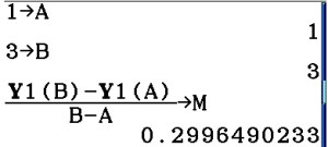
 . I entered this as Y2 in my calculator.

 for the value between a and b on your calculator. See second figure.
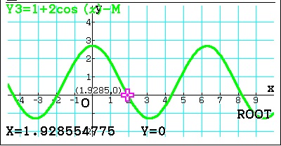
 on the home screen. See third figure.
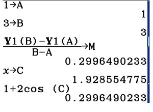
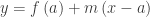
 .
.
 in step 5; set it equal to zero. Why must the solution be the value that makes
  ?
?
 .
. . The limit is
  .
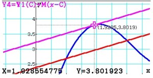
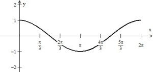
. . (See figure 1.
 is drawn.
 . (See figure 2)
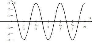
 (See figure 3. A tangent line at
  is drawn) This takes on all the values of the sine function three times between 0 and
  . It goes through the same values three times as fast and therefore, its rate of change (yeah, the derivative) should be three times as much. Compare the tangent lines in Figures 1 and 3. This agrees with the derivative found by the Chain Rule:
  . See figure 4)
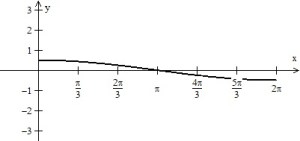
 (See figure 5. A tangent line at
  is drawn.). This time the function is stretch and only goes through half its period. So,
  (See figure 6)


 has a (removable) discontinuity at x = 3, but no value there.
 there is no value of g(3) to use, and the derivative does not exist.
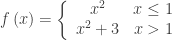 . This function has a jump discontinuity at x = 1.
 and the limit will always be a number greater than 3 divided by zero and will not exist. Therefore, even though the slopes from both side of x =1 approach the same value, namely 2, the derivative does not exist at x = 1.
 factor squeezes the function to the origin; the added condition that
  makes the function continuous. Differentiating gives
