
Unit 10 covers sequences and series. These are BC only topics (CED – 2019 p. 177 – 197). These topics account for about 17 – 18% of questions on the BC exam.
Topics 10.1 – 10.2
Topic 10.1: Defining Convergent and Divergent Series.
Topic 10. 2: Working with Geometric Series. Including the formula for the sum of a convergent geometric series.
Topics 10.3 – 10.9 Convergence Tests
The tests listed below are tested on the BC Calculus exam. Other methods are not tested. However, teachers may include additional methods.
Topic 10.3: The nth Term Test for Divergence.
Topic 10.4: Integral Test for Convergence. See Good Question 14
Topic 10.5: Harmonic Series and p-Series. Harmonic series and alternating harmonic series, p-series.
Topic 10.6: Comparison Tests for Convergence. Comparison test and the Limit Comparison Test
Topic 10.7: Alternating Series Test for Convergence.
Topic 10.8: Ratio Test for Convergence.
Topic 10.9: Determining Absolute and Conditional Convergence. Absolute convergence implies conditional convergence.
Topics 10.10 – 10.12 Taylor Series and Error Bounds
Topic 10.10: Alternating Series Error Bound.
Topic 10.11: Finding Taylor Polynomial Approximations of a Function.
Topic 10.12: Lagrange Error Bound.
Topics 10.13 – 10.15 Power Series
Topic 10.13: Radius and Interval of Convergence of a Power Series. The Ratio Test is used almost exclusively to find the radius of convergence. Term-by-term differentiation and integration of a power series gives a series with the same center and radius of convergence. The interval may be different at the endpoints.
Topic 10.14: Finding the Taylor and Maclaurin Series of a Function. Students should memorize the Maclaurin series for 
Topic 10.15: Representing Functions as Power Series. Finding the power series of a function by, differentiation, integration, algebraic processes, substitution, or properties of geometric series.
Timing
The suggested time for Unit 9 is about 17 – 18 BC classes of 40 – 50-minutes, this includes time for testing etc.
Previous posts on these topics:
Before sequences
Amortization Using finite series to find your mortgage payment. (Suitable for pre-calculus as well as calculus)
A Lesson on Sequences An investigation, which could be used as early as Algebra 1, showing how irrational numbers are the limit of a sequence of approximations. Also, an introduction to the Completeness Axiom.
Convergence Tests
Which Convergence Test Should I Use? Part 1 Pretty much anyone you want!
Which Convergence Test Should I Use? Part 2 Specific hints and a discussion of the usefulness of absolute convergence
Good Question 14 on the Integral Test
Sequences and Series
Graphing Taylor Polynomials Graphing calculator hints
New Series from Old 1 substitution (Be sure to look at example 3)
New Series from Old 2 Differentiation
New Series from Old 3 Series for rational functions using long division and geometric series
Geometric Series – Far Out An instructive “mistake.”
A Curiosity An unusual Maclaurin Series
Synthetic Summer Fun Synthetic division and calculus including finding the (finite)Taylor series of a polynomial.
Error Bounds
Error Bounds Error bounds in general and the alternating Series error bound, and the Lagrange error bound
The Lagrange Highway The Lagrange error bound.
What’s the “Best” Error Bound?
Review Notes
Type 10: Sequences and Series Questions
 and entered this in my calculator as Y1
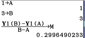
 . I entered this as Y2 in my calculator.

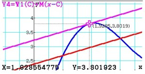
 for the value between a and b on your calculator. See second figure.
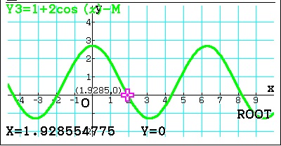
 on the home screen. See third figure.
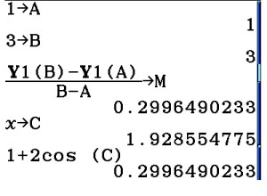
 .
.
 in step 5; set it equal to zero. Why must the solution be the value that makes
  ?
?
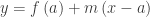
 and
and  . (Other forms may be included, but only these two are tested on the AP exams.)
 .
. . The limit is
  .
. then
then  and
and  .
. on their answer paper, so it is clear to the reader that they understand this.