Unit 3 – Differentiation: Composite, Implicit, and Inverse Function

Posted on September 21, 2021 by Lin McMullin

Unit 3 covers the Chain Rule, differentiation techniques that follow from it, and higher order derivatives. (CED – 2019 p. 67 – 77). These topics account for about 9 – 13% of questions on the AB exam and 4 – 7% of the BC questions.

Topics 3.1 – 3.6

Topic 3.1 The Chain Rule. Students learn how to apply the Chain Rule in basic situations.

Topic 3.2 Implicit Differentiation. The Chain Rule is used to find the derivative of implicit relations.

Topic 3.3 Differentiation Inverse Functions. The Chain Rule is used to differentiate inverse functions.

Topic 3.4 Differentiating Inverse Trigonometric Functions. Continuing the previous section, the ideas of the derivative of the inverse are applied to the inverse trigonometric functions.

Topic 3.5 Selecting Procedures for Calculating Derivatives. Students need to be able to choose which differentiation procedure should be used for any function they are given. This is where you can review (spiral) techniques from Unit 2 and practice those from this unit.

Topic 3.6 Calculating Higher Order Derivatives. Second and higher order derivatives are considered. Also, the notations for higher order derivatives are included here.

Topics 3.2, 3.4, and 3.5 will require more than one class period. You may want to do topic 3.6 before 3.5 and use 3.5 to practice all the differentiated techniques learned so far. The suggested number of 40 – 50-minute class periods is about 10 – 11 for AB and 8 – 9 for BC. This includes time for testing etc.

Posts on these topics include:

Foreshadowing the Chain Rule

The Power Rule Implies Chain Rule

The Chain Rule

Seeing the Chain Rule

Derivative Practice – Numbers

Derivative Practice – Graphs

Experimenting with CAS – Chain Rule

Implicit Differentiation of Parametric Equations

Adapting 2021 AB 5

This series of posts reviews and expands what students know from pre-calculus about inverses. This leads to finding the derivative of exponential functions, a^x, and the definition of e, from which comes the definition of the natural logarithm.

Inverses Graphically and Numerically

The Range of the Inverse

The Calculus of Inverses

The Derivatives of Exponential Functions and the Definition of e and This pair of posts shows how to find the derivative of an exponential function, how and why e is chosen to help this differentiation.

Logarithms Inverses are used to define the natural logarithm function as the inverse of e^x. This follow naturally from the work on inverses. However, integration is involved and this is best saved until later. I will mention it then.

Here are links to the full list of posts discussing the ten units in the 2019 Course and Exam Description.

Limits and Continuity – Unit 1 (8-11-2020)

Definition of t he Derivative – Unit 2 (8-25-2020)

Differentiation: Composite, Implicit, and Inverse Function – Unit 3 (9-8-2020) THIS POST

LAST YEAR’S POSTS – These will be updated in coming weeks

2019 CED – Unit 4 Contextual Applications of the Derivative Consider teaching Unit 5 before Unit 4

2019 – CED Unit 5 Analytical Applications of Differentiation Consider teaching Unit 5 before Unit 4

2019 – CED Unit 6 Integration and Accumulation of Change

2019 – CED Unit 7 Differential Equations Consider teaching after Unit 8

2019 – CED Unit 8 Applications of Integration Consider teaching after Unit 6, before Unit 7

2019 – CED Unit 9 Parametric Equations, Polar Coordinates, and Vector-Values Functions

2019 CED Unit 10 Infinite Sequences and Series

Differentiation: Composite, Implicit, and Inverse Function – Unit 3

Posted on September 8, 2020 by Lin McMullin

This is a re-post and update of the third in a series of posts from last year. It contains links to posts on this blog about the differentiation of composite, implicit, and inverse functions for your reference in planning. Other updated posts on the 2019 CED will come throughout the year, hopefully, a few weeks before you get to the topic. Unit 3 covers the Chain Rule, differentiation techniques that follow from it, and higher order derivatives. (CED – 2019 p. 67 – 77). These topics account for about 9 – 13% of questions on the AB exam and 4 – 7% of the BC questions.

Topics 3.1 – 3.6

Topic 3.1 The Chain Rule. Students learn how to apply the Chain Rule in basic situations.

Topic 3.2 Implicit Differentiation. The Chain Rule is used to find the derivative of implicit relations.

Topic 3.3 Differentiation Inverse Functions. The Chain Rule is used to differentiate inverse functions.

Topic 3.4 Differentiating Inverse Trigonometric Functions. Continuing the previous section, the ideas of the derivative of the inverse are applied to the inverse trigonometric functions.

Topic 3.6 Calculating Higher Order Derivatives. Second and higher order derivatives are considered. Also, the notations for higher order derivatives are included here.

Posts on these topics include:

Foreshadowing the Chain Rule

The Power Rule Implies Chain Rule

The Chain Rule

Seeing the Chain Rule

Derivative Practice – Numbers

Derivative Practice – Graphs

Experimenting with CAS – Chain Rule

Implicit Differentiation of Parametric Equations

Inverses Graphically and Numerically

The Range of the Inverse

The Calculus of Inverses

Logarithms Inverses are used to define the natural logarithm function as the inverse of e^x. This follows naturally from the work on inverses. However, integration is involved, and this is best saved until later. I will mention it then.

Here are links to the full list of posts discussing the ten units in the 2019 Course and Exam Description.

Limits and Continuity – Unit 1 (8-11-2020)

Definition of the Derivative – Unit 2 (8-25-2020)

Differentiation: Composite, Implicit, and Inverse Function – Unit 3 (9-8-2020) THIS POST

LAST YEAR’S POSTS – These will be updated in the coming weeks

2019 CED – Unit 4 Contextual Applications of the Derivative Consider teaching Unit 5 before Unit 4

2019 – CED Unit 5 Analytical Applications of Differentiation Consider teaching Unit 5 before Unit 4

2019 – CED Unit 6 Integration and Accumulation of Change

2019 – CED Unit 7 Differential Equations Consider teaching after Unit 8

2019 – CED Unit 8 Applications of Integration Consider teaching after Unit 6, before Unit 7

2019 – CED Unit 9 Parametric Equations, Polar Coordinates, and Vector-Values Functions

2019 CED Unit 10 Infinite Sequences and Series

Teaching and Learning Theorems

Posted on September 26, 2017 by Lin McMullin

Theorems are carefully worded statements about mathematical facts that have been proved to be true. Important (and some not so important) ideas in calculus and all of mathematics are summarized as theorems. When you come across a theorem you need to understand it; the author of your textbook would not have included it and the AP Exams would not test it if it were not. This post discusses some things about theorems in general. Students often do not realize these things; understanding them will help students understand a new theorem when it is presented to them.

Theorems have the form of IF one or more things are true (called the hypothesis), THEN some other thing is true (called the conclusion). This is abbreviated $p\to q$ where p represents the hypothesis and q represents the conclusion. This is read as “if p, then q” or “p implies q.” Theorems are also known as conditional statements.

In a certain instance, once you are sure all the conditions of the hypothesis are true, then you may be absolutely certain the conclusion is also true. When trying to determine if something is true about some function, check to see if the conditions of the hypothesis are all true.

People using a theorem need to know the hypotheses as well as the conclusion.

When teaching about a particular theorem, one thing that is often helpful to students is to “play” with the hypothesis and see how it affects the conclusion. For instance, if the hypothesis requires a function to be continuous, see what happens if the function is not continuous. If there are several parts to the hypothesis, see what happens if one or the other is changed. Hint: A change in part of the hypothesis will make some difference – good theorems do not have extra, unneeded, or superfluous conditions.

To make them read better, some theorems are not stated in if …, then… form. If there is any confusion, restate the theorem in if…, then… form.

The theorem often stated as, “Differentiability implies continuity,” really means: IF a function is differentiable at a point, THEN it is continuous at that point.
The geometry theorem, “The diagonals of a rhombus are perpendicular,” really means: IF a quadrilateral is a rhombus, THEN its diagonals are perpendicular.

The Contrapositive

Since if p is true, q must be true, what happens if q is false? The answer is that p must also be false. This is a related conditional statement (theorem) called the contrapositive of the theorem. The contrapositive is abbreviated IF not q, THEN not p, or IF q is false, THEN p is false, or $\tilde{\ }q\to \tilde{\ }p$ . The contrapositive of a theorem is also true, always.

There are several theorems in the calculus where the contrapositive seems to be used more often than the theorem itself.

Differentiability implies continuity. The contrapositive of this theorem is: IF a function is not continuous at a point, THEN it is not differentiable at that point. This is a quick way to tell if a function is not differentiable.
IF an infinite series converges, THEN the limit as n goes to infinity of its n^th term is zero. Here the contrapositive is IF the limit as n goes to infinity of its n^th term of an infinite series is not zero, THEN the series does not converge. This is called the n^th term test for divergence.
IF the diagonals of a quadrilateral are not perpendicular, THEN the quadrilateral is not a rhombus.

The converse

The converse of a theorem is a statement formed by switching the hypothesis and conclusion of the theorem: IF q, THEN p (or $q\to p$ ). The converse is not necessarily true. It may be true, in which case it need to be proved as a separate theorem. Students (among others) often assume that the converse is true – this is called the fallacy of the converse.

IF a function is continuous at a point, THEN it is differentiable there, is the converse of our previous example. It is false: a simple counterexample is f(x) = |x|. This function is continuous at the origin but not differentiable there.
Another theorem states that IF the derivative of a function is positive on an interval, THEN the function is increasing on the interval. The converse is, IF a function is increasing on an interval, THEN its derivative is positive on the interval. The converse is false: for example, f(x) = x³ is increasing everywhere, yet its derivative at the origin is zero. (See Going up?)
IF the diagonals of a quadrilateral are perpendicular, Then the quadrilateral is a rhombus, if false. The quadrilateral may have perpendicular diagonals, but unless they intersect at their midpoints the figure is not a rhombus (it is a kite shape).

The inverse

The inverse is the contrapositive of the converse or IF not p, THEN not q (or $\tilde{\ }p\to \tilde{\ }q$ ). The inverse will be true if the converse is true, and false if the converse is false.

The inverse of our fist example is,IF a function is not differentiable on an interval, THEN it is not continuous there. This is false, since the function my fail to be differentiable even though it is continuous. An example is f(x) = |x|. again.
IF a quadrilateral is not a rhombus, THEN he diagonals are not perpendicular (false – the kite again).

Biconditional statements

A biconditional theorem is a theorem whose converse is also true (and therefore its inverse and contrapositive are true). These are written in the form p if, and only if, q or $p\leftrightarrow q$ (or for that matter $q\leftrightarrow p$ ). It is equivalent to $p\to q\text{ and }q\to p$ .

An example from Geometry: IF two sides of a triangle are congruent, THEN the angles opposite them are congruent. The converse of this theorem is, if two angles of a triangle are congruent,THEN the sides opposite them are congruent. Since both the theorem and its converse (and its inverse, and its contrapositive) are true, you may write, “Two sides of a triangle are congruent if, and only if, the angles opposite them are congruent.”

Definitions are always biconditional statements. They are always true and do not need to be proved; in fact they cannot be proved.

The definition of continuous at a point is, “A function is continuous at a point $\left( {a,f\left( a \right)} \right)$ if, and only if, $\underset{{x\to a}}{\mathop{{\lim }}}\,f\left( x \right)=f\left( a \right)$ and both the limit and value are finite.”
A rectangle is defined as a quadrilateral with four right angles or A quadrilateral is a rectangle if, and only if, it has four right angles.

Which is which?

The theorem, its contrapositive, converse, and inverse are all theorems. Any of them could be taken as “the theorem” and the others would rearrange their names accordingly. (Which is good practice for your students.)

One other thing

What if the hypothesis of a theorem is false: can the conclusion still be true? The answer is, yes! The hypothesis of a theorem tells us that if true, the conclusion must be true. But the conclusion may be true anyway.

Consider the Mean Vale Theorem (MVT): IF a function, f, is continuous on the closed interval [a, b] and differentiable on the open interval (a, b), THEN there exists at least one number c in the open interval (a, b) such that $\displaystyle {f}'\left( c \right)=\frac{{f\left( b \right)-f\left( a \right)}}{{b-a}}$ .

But consider the function $f\left( x \right)=\left\{ {\begin{array}{*{20}{c}} {{{x}^{2}}} & {-2\le x\le 1} \\ \text{4} & {1<x\le 2} \end{array}} \right.$
This function has a jump discontinuity at x = 1 and therefore is neither continuous nor differentiable on the interval [-2, 2]; the MVT does not apply. Yet $\displaystyle {f}'\left( 0 \right)=\frac{{f\left( 2 \right)-f\left( {-2} \right)}}{{2-\left( {-2} \right)}}=\frac{{4-4}}{4}=0$ . (In fact, c could be 0 or any number between 1 and 2). In this example and not every example, the conclusion of the MVT is true even though the hypothesis is false.
On the 2017 International exam AB 15 makes use of the idea that even though the theorem about limits that seems to apply doesn’t because the conditions are not met, but, nevertheless, the conclusion is true.

Proof

The proofs of all the important theorems are given in any good textbook. You study proofs for two reasons: (1) to see why a theorem is true, and (2) to learn how to write a proof of your own. If neither of these reasons concern you or your students (and they may not), then you still need to learn the hypothesis and conclusion, and how to apply the theorem. This cannot be avoided.

Some proofs are rather tricky. That is, the key step is not obvious. A beginning calculus student should not expect to know how to prove most of the theorems; they should, however, be able to follow the proofs in the textbook. The AP Calculus exams never ask for proof, per se, although they may ask you to justify a conclusion you make. The justification should show that the hypotheses are all true and state the name of the theorem that implies your conclusion.

I can recall only one time many years ago where students were asked to “prove” something on an AP Calculus Exam. The usual instruction is “Justify your answer” or “Explain your reasoning.” This means that students are supposed to cite the appropriate theorem and show that the hypotheses are met in the given situation. So, not quite “prove” but close. It’s not “prove” an original theorem, but rather determine which (unnamed) theorem applies (or does not apply) in a particular situation and verify that the conditions are (or are not) met.

As always, look at a number of past exams and see just what is asked and how it is asked.

Inverses Graphically and Numerically

Posted on November 14, 2012 by Lin McMullin

In this final post in this series on inverses we consider the graphical and numerical concepts related to the derivative of the inverse and look at an important formula.

To make the notation a little less messy, let’s let g(x) = f ^-1(x). Then we know that f (g(x))= x. Differentiating this implicitly gives

${f}'\left( g\left( x \right) \right){g}'\left( x \right)=1$
$\displaystyle {g}'\left( x \right)=\frac{1}{{f}'\left( g\left( x \right) \right)}$

Great formula, but one I’ve never been able to memorize and use correctly! It’s my least favorite formula, because I’m never quite sure what to substitute for what.

The graph shows a function and its inverse. It really doesn’t matter which is which, since inverse functions come in pairs: the inverse of the inverse is the original function.

Notice that the graphs are symmetric to y = x. At two points, one of which is the image of the other after reflecting over the line y = x, a tangent segment has been drawn. This segment is the hypotenuse of the “slope triangle” which is also drawn. The ratio of the vertical side of this triangle to the horizontal side is the slope (i.e. the derivative) of the tangent line.

The two triangles are congruent, so that the horizontal side of one triangle is congruent to the vertical side of the other, and vice versa. Thus the slope (the derivative) of the one tangent segment is the reciprocal of the other.

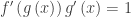
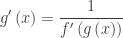
If (a, b) is a point on a function and the derivative at this point is ${f}'\left( a \right)$ , then the point (b, a) is on the function’s inverse and the derivative here is $\displaystyle \frac{1}{{f}'\left( a \right)}$ . This is just what my least favorite formula says: if f ^-1 (x) = g(x), then a = g(b) and $\displaystyle {g}'\left( b \right)=\frac{1}{{f}'\left( a \right)}=\frac{1}{{f}'\left( g\left( b \right) \right)}$ .

What you really need to know is:

At corresponding points on a function and its inverse, the derivatives are reciprocals of each other.

This is what my least favorite formula says.

The AP exams have a clever way of testing this. (The stem may give a few more values to throw you off, or the values may be in a table.)

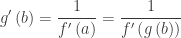Given that $f\left( 2 \right)=5\text{ and }{f}'\left( 2 \right)=3$ and g is the inverse of f, Find ${g}'\left( 5 \right)$ .

The solution is reasoned this way: (5, ?) is a point on g. The corresponding point on f is (?, 5) = (2, 5). The derivative of f at this point is 3, therefore the derivative at (5, 2) on g is ${g}'\left( 5 \right)=\tfrac{1}{3}$ .

Easy!

The Calculus of Inverses

Posted on November 12, 2012 by Lin McMullin

Today we will consider computing the derivative of the inverse of a function. This is pretty standard and is in all the textbooks.

The usual suspects are the inverse trigonometric functions. So let’s start with $y={{\sin }^{-1}}\left( x \right)$ and then rewrite this as $x=\sin \left( y \right)$ . Differentiating this gives

$\displaystyle 1=\cos \left( y \right)\frac{dy}{dx}$
$\displaystyle \frac{dy}{dx}=\frac{1}{\cos \left( y \right)}$

Since we would like this in terms of x we can proceed two ways.

The denominator is the cosine of the number whose sine is x. So using the relationship

$\cos \left( y \right)=\sqrt{1-{{\sin }^{2}}\left( y \right)}=\sqrt{1-{{x}^{2}}}$

we find that

$\displaystyle \frac{dy}{dx}=\frac{1}{\sqrt{1-{{x}^{2}}}}$ .

That tends to be confusing so another method is to draw a right triangle with an acute angle of y and arrange the side so that

$\displaystyle \sin \left( y \right)=\frac{x}{1}=\frac{\text{opposite}}{\text{hypotenuse}}$

From this we can find all the trigonometric functions of y, specifically:

$\displaystyle \cos \left( y \right)=\frac{\text{adjacent}}{\text{hypotenuse}}-\frac{\sqrt{1-{{x}^{2}}}}{1}=\sqrt{1-{{x}^{2}}}$ and $\displaystyle \frac{dy}{dx}=\frac{1}{\sqrt{1-{{x}^{2}}}}$ .

A second example: Find the derivative of $y={{\sec }^{-1}}\left( x \right)$ . The domain of this function is $\left| x \right|\ge 1$ and the range is $[0,\tfrac{\pi }{2})\cup (\tfrac{\pi }{2},\pi ]$ , the function is increasing on both parts of its domain; we will need to know this.

Proceeding as above we will find that

$\displaystyle \frac{dy}{dx}=\frac{1}{\sec \left( y \right)\tan \left( y \right)}$ .

Drawing a triangle as above and arranging the side so that sec(y) = x:

Then $\displaystyle \frac{dy}{dx}=\frac{1}{x\sqrt{1+{{x}^{2}}}}$ ,

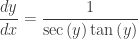But wait! It may be that x < 0, but ${{\sec }^{-1}}\left( x \right)$ is increasing and the derivative should always be positive. So, this needs to be adjusted to

$\displaystyle \frac{d}{dx}{{\sec }^{-1}}\left( x \right)=\frac{1}{\left| x \right|\sqrt{1+{{x}^{2}}}}$

These can be a bit tricky.

Next: the fifth and last posting in this series will look at the graphical and numerical aspects of the derivatives of a function and its inverse.

The Range of the Inverse

Posted on November 9, 2012 by Lin McMullin

The last two post discussed inverse functions and some concerns about them. We continue that today be considering that fact that sometimes the inverse of a function is not a function, and what can be done in that case.

Since the square of both 3 and –3 is 9. Which number should you get when you unsquare 9? Is the result, 3 or –3?

Mathematicians want, for practical reasons, inverses to be functions. If the original function is not strictly monotonic then the inverse will not be a function. That is, if there are places on the original function that have the same y-values then the inverse (set of ordered pairs found by reversing the function’s ordered pairs) will not be a function. If some horizontal line intersects the graph of the function more than once, the inverse will not be a function.

While it may seem a bit too convenient, what is done is that the range of the inverse is restricted so that the inverse is a function. So for f (x) = x² the range of the inverse is restricted to non-negative values. So f^-1(9) = 3 and f^-1(10) = $\sqrt{10}$ where it is understood that this represents a non-negative number. This is why 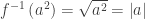${{f}^{-1}}\left( {{a}^{2}} \right)=\sqrt{{{a}^{2}}}=\left| a \right|$ . So that if a = –4, $\sqrt{{{a}^{2}}}=\left| -4 \right|=4$ .

The restriction is arbitrary. It would be just as possible to make the range all non-positive numbers. While arbitrary, the restriction is not unreasonable. After all, once we understand this, we can easily find the other value if we need it. This is also necessary for calculators to work; the process they use to compute the value can only return one value. The (restricted) ranges of the common functions are what mathematicians feel are the most useful.

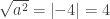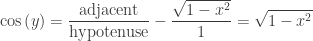
None of the trigonometric functions pass the horizontal line test; none of their inverses are functions until the ranges have been restricted. These restrictions are in the textbooks. For example: The domain of sin^-1(x) is $-1\le x\le 1$ , these are the output values of the sin(x); the range is restricted to 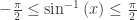$\displaystyle -\tfrac{\pi }{2}\le {{\sin }^{-1}}\left( x \right)\le \tfrac{\pi }{2}$ . Because the signs of the trig functions are different outside of the first quadrant and in order to make as many of the inverses as possible continuous, each inverse trig function has a different range. You will find these in your textbook. They are built into calculators and computers. This can be a little confusing for students, but there is not much that can be done about that.

This is the third of 5 posts on inverses. The next post: The Calculus of Inverses.

Writing Inverses

Posted on November 7, 2012 by Lin McMullin

In my last post I identified two “problems” related to inverses. The first of these is that there may be no string of operations, no algebra or arithmetic, which tells us how to evaluate the inverse function.

For simple functions you can find the inverse function by switching the x and the y and then solving for y. If you can do that, this produces a nice expression for the inverse. Alas usually you cannot do that.

What to do?

What you can do is invent a name and/or a symbol for the new function. So if f(x) = x², we write f^-1(x) = $\sqrt{x}$ and we think we have solved the problem. We have not. While I can write $\sqrt{x}$ , what arithmetic can I do to express this number as a decimal? There is an algorithm for this; (you can find it on the internet by searching for “square root algorithm”). You can use a calculator or look in a table as we did back in the “old days.” But that is not the same as performing a series of arithmetic or algebraic operations.

And if $\sqrt{10}$ does not slow you down, how about sin^-1(0.12345)? The only hope in some cases is to try to solve something like x² = 10 or sin(y) = 0.12345, not much hope there. We are left with using technology of some sort if we need a number (decimal); calculators have buttons for square roots and inverse sines. But sometimes writing $\sqrt{10}$ or sin^-1(0.12345) is good enough.

Making up a new function or symbol to “solve” a problem, even if that function cannot be written as a string of operations is actually fairly common. The sin(x) is defined as the y-coordinate of a point on the unit circle. Except for some special numbers you cannot find y-coordinates that easily. You have seen others already. All the trigonometric functions and their inverses as well as logarithmic functions are of this sort. Mathematics is full of them.

The next post will discuss the other problem: the inverse of a function may not be a function. Since there are two numbers whose square is 9, what is the “unsquare” of 9; is it 3 or –3?

This is the second of 5 posts on inverses.

Teaching Calculus

The pleasure lies not in discovering the truth, but in searching for it.

Tag Archives: Inverse

Unit 3 – Differentiation: Composite, Implicit, and Inverse Function

Topics 3.1 – 3.6

Differentiation: Composite, Implicit, and Inverse Function – Unit 3

Topics 3.1 – 3.6

Teaching and Learning Theorems

Inverses Graphically and Numerically

The Calculus of Inverses

The Range of the Inverse

Writing Inverses

Topics 3.1 – 3.6

Share this:

Like this:

Topics 3.1 – 3.6

Share this:

Like this:

Share this:

Like this:

Share this:

Like this:

Share this:

Like this:

Share this:

Like this:

Share this:

Like this: