Good Question 1: 2008 AB 6

Posted on January 21, 2015 by Lin McMullin

When I started this blog several years ago I was hoping my readers would ask questions that we could discuss or submit ideas for additional topics to write about. This has not really happened, but I’m still very open to the idea. (That was a HINT.) Since that first year when I had the entire curriculum ahead of me, I have written less not because I dislike writing, but because I am low on ideas.

The other day, I answered a question posted on the AP Calculus Community bulletin board about AB calculus exam question. It occurred to me that this somewhat innocuous looking question was quite good. So I decided to start an occasional series on good questions, from AP exams or elsewhere, that can be used to teaching beyond the actual things asked in the question. (My last post might be in this category, but that was written several months ago.)

In discussing these questions, I will make numerous comments about the question and how to take it further in your class. My idea is not just to show how to write a good answer, but rather to use the question to look deeper into the concepts involved.

Good Question #1: 2008 AB Calculus exam question 6.

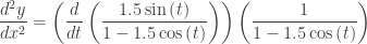
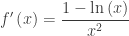
The stem gave students the function $\displaystyle f\left( x \right)=\frac{\ln \left( x \right)}{x},\quad x>0$ . Students were also told that $\displaystyle {f}'\left( x \right)=\frac{1-\ln \left( x \right)}{{{x}^{2}}}$ .

The first thought that occurs is why they gave the derivative. The reason is, as we will see, that the first derivative is necessary to answer the first three parts of the question. Therefore, a student who calculates an incorrect derivative is going to be in big trouble (and the readers may have a great deal of work to do reading with the student’s incorrect work). The derivative is calculated using the quotient rule, and students will have to demonstrate their knowledge of the quotient rule later in this question; there is no reason to ask them to do the same thing twice.
If you are using this with a class, you can, and probably should, ask your students to calculate the first derivative. Then you can see how many giving the derivative would have helped.
When discussing the stem, you should also discuss the domain, x > 0, and the x-intercept (1, 0). Other features of the graph, such as end behavior, are developed later in the question, so they may be put on hold briefly.

Part a asked students to write an equation of the tangent line at x = e². To do this students need to do two calculations: $\displaystyle f\left( {{e}^{2}} \right)=\frac{2}{{{e}^{2}}}$ and $\displaystyle {f}'\left( {{e}^{2}} \right)=-\frac{1}{{{e}^{4}}}$ . An equation of the tangent line is $\displaystyle y=\frac{2}{{{e}^{2}}}-\frac{1}{{{e}^{4}}}\left( x-{{e}^{2}} \right)$ .

Writing the equation of a tangent line is a very important skill and should be straightforward. The point-slope form is the way to go. Avoid slope-intercept.
The tangent line is used to approximate the value of the function near the point of tangency; you can throw in an approximation computation here.
After doing part c, you should return here and discuss whether the approximation is an overestimate or an underestimate and how you can tell. (Answer: underestimate, since the graph is concave up here.)
After doing part c, you can also ask them to write the tangent line at the point of inflection and whether approximations near the point of inflection are overestimates or an underestimates, and why. (Answer: Since the concavity change here, it depends on which side of the point of inflection the approximation is made. To the left is an overestimate; to the right is an underestimate.)

Part b asked students to find the x-coordinate of the critical point, determine whether it is a maximum, a minimum, or neither, and to “justify your answer.” To earn credit students had to write the equation $\displaystyle {f}'\left( x \right)=0$ and solve it getting x = e. They had to state that this is a maximum because “ ${f}'\left( x \right)$ changes from positive to negative at x = e.”

This is a very standard AP exam question. To expand it in your class:

Discuss how you know the derivative changes sign here. This will get you into the properties of the natural logarithm function.
Discuss why the change in sign tells you this is a maximum. (A positive derivative indicates an increasing function, etc.)
After doing part c, you can return here and try the second derivative test.
The question asks for “the” critical point, hinting that there is only one. Students should learn to pick up on hints like this and be careful if their computation produces more or less than one.
At this point we have also determined that the function is increasing on the interval $\left( -\infty ,e \right]$ and decreasing everywhere else. The question does not ever ask this, but in class this is worth discussing as important features of the graph. On why these are half-open intervals look here.

Part c told students there was exactly one point of inflection and asked them to find its x-coordinate. To do this they had to use the quotient rule to find that $\displaystyle {{f}'}'\left( x \right)=\frac{-3+2\ln \left( x \right)}{{{x}^{3}}}$ , set this equal to zero and find the x-coordinate to be x = e^3/2.

The question did not require any justification for this answer. In class you should discuss what a justification would look like. The reason is that the second derivative changes sign here. So now you need to discuss how you know this.
Also, you can now determine that the function is concave down on the interval $\left( -\infty ,{{e}^{3/2}} \right)$ and concave up on the interval $\left({{e}^{3/2}},\infty \right)$ . Ask your class to justify this.

Part d asked student to find $\displaystyle \underset{x\to 0+}{\mathop{\lim }}\,\frac{\ln \left( x \right)}{x}$ . The answer is $-\infty$ . While this seems almost like a throwaway tacked on the end because they needed another point, it is the reason I like this question.

The question is easily solved: $\displaystyle \underset{x\to 0+}{\mathop{\lim }}\,\frac{\ln \left( x \right)}{x}=\underset{x\to 0+}{\mathop{\lim }}\,\frac{1}{x}\cdot \underset{x\to 0+}{\mathop{\lim }}\,\ln \left( x \right)=\left( \infty \right)\left( -\infty \right)=-\infty$ .
While tempting, the limit cannot be found by L’Hôpital’s Rule, because on substitution you get $\frac{-\infty }{0}$ ,which is not one of the forms that L’Hôpital’s Rule can handle.
The reason I like this part so much is that we have already developed enough information in the course of doing the problem to find this limit! The function is increasing and concave down on the interval $\left( -\infty ,e \right)$ . Moving from the maximum to the left, the function crosses the x-axis at (1, 0), keeps heading south, and gets steeper. So the limit as you approach the y-axis from the right is negative infinity.This is the left-side end behavior.
What about the right-side end behavior? (You ask your class.) Well, the function is positive and decreasing to the right of the maximum and becomes concave up after x = e^3/2. Thus, it must flatten out and approach the x-axis as an asymptote.
That $\displaystyle \underset{x\to \infty }{\mathop{\lim }}\,\frac{\ln \left( x \right)}{x}=0$ is clear from the note immediately above. This limit can be found by L’Hôpital’s Rule since it is an indeterminate of the type $\infty /\infty$ . So, $\displaystyle \underset{x\to \infty }{\mathop{\lim }}\,\frac{\ln \left( x \right)}{x}=\underset{x\to \infty }{\mathop{\lim }}\,\frac{\tfrac{1}{x}}{1}=0$ .
Notice also that the first derivative approaches zero as x approaches infinity. This indicates that the function’s graph approaches the horizontal as you travel farther to the right. The second derivative also approaches zero as x approaches infinity indicating that the function’s graph is becoming flatter (less concave).

This question and the discussion is largely done analytically (working with equations). We did find a few important numbers in the course of the work. Hopefully, you students discussed this with many good words. To complete the Rule of Four, here is the graph.

And here is a close up showing the important features of the graph and the corresponding points on the derivatives.

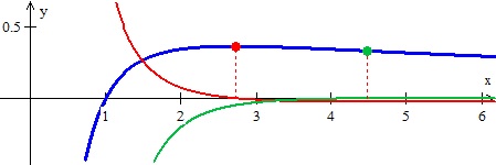
The function is shown in blue, the derivative and maximum in red, and the second derivative and the point of inflection in green.

Finally, this function and the limit at infinity is similar to the more pathological example discussed in the post of October 31, 2012 entitled Far Out!

A Vector’s Derivatives

Posted on January 14, 2015 by Lin McMullin

A question on the AP Calculus Community bulletin board this past Sunday inspired me to write this brief outline of what the derivatives of parametric equations mean and where they come from.

The Position Equation or Position Vector

A parametric equation gives the coordinates of points (x, y) in the plane as functions of a third variable, usually t for time. The resulting graph can be thought of as the locus of a point moving in the plane as a function of time. This is no different than giving the same two functions as a position vector, and both approaches are used. (A position vector has its “tail” at the origin and its “tip” tracing the path as it moves.)

For example, the position of a point on the flange of a railroad wheel rolling on a horizontal track (called a prolate cycloid) is given by the parametric equations

$x\left( t \right)=t-1.5\sin \left( t \right)$

$y\left( t \right)=1-1.5\cos \left( t \right)$ .

Or by the position vector with the same components $\left\langle t-1.5\sin \left( t \right),1-1.5\cos \left( t \right) \right\rangle$ .

Derivatives and the Velocity Vector

The instantaneous rate of change in the y-direction is given by dy/dt, and dx/dt gives the instantaneous rate of change in the x-direction. These are the two components of the velocity vector $\displaystyle \vec{v}\left( t \right)=\left\langle \frac{dx}{dt},\frac{dy}{dt} \right\rangle$ .

In the example, $\displaystyle \vec{v}\left( t \right) =\left\langle 1-1.5\cos \left( t \right),1.5\sin \left( t \right) \right\rangle$ . This is a vector pointing in the direction of motion and whose length, $\displaystyle \sqrt{{{\left( \frac{dx}{dt} \right)}^{2}}+{{\left( \frac{dy}{dt} \right)}^{2}}}$ , is the speed of the moving object.

In the video below the black vector is the position vector and the red vector is the velocity vector. I’ve attached the velocity vector to the tip of the position vector. Notice how the velocitiy’s length as well as its direction changes. The velocity vector pulls the object in the direction it points and there is always tangent to the path. This can be seen when the video pauses at the end and in the two figures at the end of this post.

The slope of the tangent vector is the usual derivative dy/dx. It is found by differentiating dy/dt implicitly with respect to x. Therefore, $\displaystyle \frac{dy}{dx}=\frac{dy}{dt}\cdot \frac{dt}{dx}$ .

There is no need to solve for t in terms of x since dt/dx is the reciprocal of dx/dt, instead of multiplying by dt/dx we can divide by dx/dt: $\displaystyle \frac{dy}{dx}=\frac{dy/dt}{dx/dt}$ .

In the example, $\displaystyle \frac{dy}{dx}=\left( 1.5\sin \left( t \right) \right)\frac{dt}{dx}=\left( 1.5\sin \left( t \right) \right)\left( \frac{1}{1-1.5\cos \left( t \right)} \right)=\frac{1.5\sin \left( t \right)}{1-1.5\cos \left( t \right)}$

Second Derivatives and the Acceleration Vector

The components of the acceleration vector are just the derivatives of the components of the velocity vector

In the example, $\displaystyle \vec{a}\left( t \right)=\left\langle 1.5\sin \left( t \right),1.5\cos \left( t \right) \right\rangle$

The usual second derivative $\displaystyle \frac{{{d}^{2}}y}{d{{x}^{2}}}$ is found by differentiating dy/dx, which is a function of t, implicitly with respect to x:

$\displaystyle \frac{{{d}^{2}}y}{d{{x}^{2}}}=\left( \frac{d}{dt}\left( \frac{dy}{dx} \right) \right)\left( \frac{dt}{dx} \right)=\frac{\frac{d}{dt}\left( dy/dx \right)}{dx/dt}$

In the example,

$\displaystyle \frac{{{d}^{2}}y}{d{{x}^{2}}}=\left( \frac{d}{dt}\left( \frac{1.5\sin \left( t \right)}{1-1.5\cos \left( t \right)} \right) \right)\left( \frac{1}{1-1.5\cos \left( t \right)} \right)$

$\displaystyle =\frac{\left( 1-1.5\cos \left( t \right) \right)\left( 1.5\cos \left( t \right) \right)-\left( 1.5\sin \left( t \right) \right)\left( 1.5\sin \left( t \right) \right)}{{{\left( 1-1.5\cos \left( t \right) \right)}^{2}}}\cdot \frac{1}{\left( 1-1.5\cos \left( t \right) \right)}$

$\displaystyle =\frac{1.5\cos \left( t \right)-{{1.5}^{2}}}{{{\left( 1-1.5\cos \left( t \right) \right)}^{3}}}$

The acceleration vector is the instantaneous rate of change of the velocity vector. You may think of it as pulling the velocity vector in the same way as the velocity vector pulls the moving point (the tip of the position vector). The video below shows the same situation as the first with the acceleration vectors in green attached to the tip of the velocity vector.

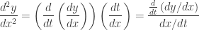
Here are two still figures so you can see the relationships. On the left is the starting position t = 0 with the y-axis removed for clarity. At this point the red velocity vector is $\left\langle -0.5,0 \right\rangle$ indicating that the object will start by moving directly left. The green acceleration vector is $\left\langle 0,1.5 \right\rangle$ pulling the velocity and therefore the object directly up. The second figure shows the vectors later in the first revolution. Note that the velocity vector is in the direction of motion and tangent to the path shown in blue.

The Marble and the Vase

Posted on October 23, 2014 by Lin McMullin

A fairly common max/min problem asks the student to find the point on the parabola $f\left( x \right)={{x}^{2}}$ that is closest to the point $A\left( 0,1 \right)$ . The solution is not too difficult. The distance, L(x), between A and the point $\left( x,{{x}^{2}} \right)$ on the parabola is given by

$\displaystyle L\left( x \right)=\sqrt{{{\left( x-0 \right)}^{2}}+{{\left( {{x}^{2}}-1 \right)}^{2}}}=\sqrt{{{x}^{4}}-{{x}^{2}}+1}$

And the minimum distance can be found when

$\displaystyle \frac{dL}{dx}=\frac{4{{x}^{3}}-2x}{2\sqrt{{{x}^{4}}-{{x}^{2}}+1}}=0$

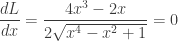
This occurs when $x=0,\frac{1}{\sqrt{2}},-\frac{1}{\sqrt{2}}$ . The local maximum is occurs when x = 0. The (global) minimums are the other two values located symmetrically to the y-axis.

_________________________

Somewhere I saw this problem posed in terms of a marble dropped into a vase shaped like a parabola. So I think of it that way. This accounts for the title of the post. The problem is, however, basically a two-dimensional situation.

In this post I would like to expand and explore this problem. The exploration will, I hope, give students some insight and experience with extreme values, and the relationship between a graph and its derivative. I will pose a series of questions that you could give to your students to explore. I will answer the questions as I go, but you, of course, should not do that until your students have had some time to work on the questions.

Graphing technology and later Computer Algebra Systems (CAS) will come in handy.

_________________________

1. Consider a general point $A\left( 0,a \right)$ on the y-axis. Find the x-coordinates of the closest point on the parabola in terms of a.

The distance is now given by

$\displaystyle L\left( x \right)=\sqrt{{{\left( x-0 \right)}^{2}}+{{\left( {{x}^{2}}-a \right)}^{2}}}=\sqrt{{{x}^{4}}+\left( 1-2a \right){{x}^{2}}+{{a}^{2}}}$

$\displaystyle \frac{dL}{dx}=\frac{2{{x}^{3}}+\left( 1-2a \right)x}{\sqrt{{{x}^{4}}+2\left( 1-2a \right){{x}^{2}}+{{a}^{2}}}}$

And $\frac{dL}{dx}=0$ when $x=0,\frac{\sqrt{2\left( 2a-1 \right)}}{2},-\frac{\sqrt{2\left( 2a-1 \right)}}{2}$

The (local) maximum is at x = 0. The other values are the minimums. The CAS computation is shown at the end of the post. This is easy enough to do by hand.

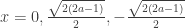
2. Discuss the equation ${{L}^{2}}={{x}^{2}}+{{\left( x-a \right)}^{2}}$ in relation to this situation.

This is the equation of a circle with center at A with radius of L. At the minimum distance this circle will be tangent to the parabola.

3. What happens when $a=\tfrac{1}{2}$ and when $a<\tfrac{1}{2}$ ?

When $a=\tfrac{1}{2}$ , the three zeroes are the same. The circle is tangent to the parabola at the origin and a is the minimum distance.

When $a<\tfrac{1}{2}$ , the circle does not intersect the parabola. Notice that in this case two of the roots of $\frac{dL}{dt}=0$ are not Real numbers.

4. Consider the distance, L(x), from point A to the parabola. As x moves from left to right describe how this length changes. Be specific. Sketch the graph of this distance y = L(x). Where are its (local) maximum and minimum values, relative to the parabola and the circle tangent to the parabola?

The clip below illustrates the situation. The two segments marked L(x) are congruent. The graph of y = L(x) is a“w” shape similar to but not quartic polynomial. The minimums occur directly under the points of tangency of the circle and the parabola. The local maximum is directly over the origin. Is it coincidence that the graph goes through the center of the circle? Explain.

5. Graph $y=\frac{dL}{dx}$ and compare its graph with the graph of $y=L(x)$

L(x) is the blue graph and and L'(x) is the orange graph.
Notice the concavity of L'(x)

6. The graph of $y=\frac{dL}{dx}$ appears be concave up, then down, then (after passing the origin) up, and then down again. There are three points of inflection. Find their x-coordinates in terms of a. How do these points relate to y = L(x) ? (Use a CAS to do the computation)

The points of inflection of the derivative can be found from the second derivative of the derivative (the third derivative of the L(x)). The abscissas are $x=-\sqrt{a},x=0,\text{ and }\sqrt{a}$ . The CAS computation is shown below

CAS Computation for questions 1 and 6.

Power Rule Implies Chain Rule

Posted on September 20, 2014 by Lin McMullin

Having developed the Product Rule $d\left( uv \right)=u{v}'+{u}'v$ and the Power Rule $\frac{d}{dx}{{x}^{n}}=n{{x}^{n-1}}$ for derivatives in your class, you can explore similar rules for the product of more than two functions and suddenly the Chain Rule will appear.

For three functions use the associative property of multiplication with the rule above:

$d\left( uvw \right)=d\left( \left( uv \right)w \right)=u\cdot v\cdot dw+w\cdot d(uv)=u\cdot v\cdot dw+w\left( udv+vdu \right)$

So expanding with a slight change in notation:

$d\left( uvw \right)=uv{w}'+u{v}'w+u'vw$

For four factors there is a similar result:

$d\left( uvwz \right)=uvw{z}'+uv{w}'z+u{v}'wz+{u}'vwz$

Exercise: Let ${{f}_{i}}$ for $i=1,2,3,...,n$ be functions. Write a general formula for the derivative of the product ${{f}_{1}}{{f}_{2}}{{f}_{3}}\cdots {{f}_{n}}$ as above and in sigma notation

Answers

$d\left( {{f}_{1}}{{f}_{2}}{{f}_{3}}\cdots {{f}_{n}} \right)={{f}_{1}}{{f}_{2}}{{f}_{3}}\cdots {{{f}'}_{n}}+{{f}_{1}}{{f}_{2}}{{{f}'}_{3}}\cdots {{f}_{n}}+{{f}_{1}}{{{f}'}_{2}}{{f}_{3}}\cdots {{f}_{n}}+\cdots +{{{f}'}_{1}}{{f}_{2}}{{f}_{3}}\cdots {{f}_{n}}$

$\displaystyle d\left( {{f}_{1}}{{f}_{2}}{{f}_{3}}\cdots {{f}_{n}} \right)=\sum\limits_{i=1}^{n}{\frac{{{f}_{1}}{{f}_{2}}{{f}_{3}}\cdots {{f}_{n}}}{{{f}_{i}}}{{{{f}'}}_{i}}}$

This idea may now be used to see the Chain Rule appear. Students may guess that $d{{\left( f \right)}^{4}}=4{{\left( f \right)}^{3}}$ , but wait there is more to it.

Write ${{\left( f \right)}^{4}}=f\cdot f\cdot f\cdot f\text{ }$ . Then from above

$d{{\left( f \right)}^{4}}=d\left( f\cdot f\cdot f\cdot f\text{ } \right)=f\cdot f\cdot f\cdot {f}'+f\cdot f\cdot {f}'\cdot f+f\cdot {f}'\cdot f\cdot f+{f}'\cdot f\cdot f\cdot f$

$d{{\left( f \right)}^{4}}=4{{\left( f \right)}^{3}}{f}'\text{ }$

Looks just like the power rule, but there’s that “extra” ${f}'$ . Now you are ready to explain about the Chain Rule in the next class.

Mean Tables

Posted on September 16, 2014 by Lin McMullin

The AP calculus exams always seem to have a multiple-choice table question in which the stem describes function in words and students are asked which of 5, now 4, tables could be a table of values for the function. Could be because you can never be sure without other information what happens between values in the table. So, the way to solve the problem is to eliminate choices that are at odds with the description.

The question style nicely makes students relate a verbal description with the numerical information in the tables. This uses two parts of the Rule of Four.

In 2003, question AB 90 told students that a function f had a positive first derivative and a negative second derivative on the closed interval [2, 5]. There were five tables to choose from.

There is a fairly quick way to solve the problem, but I want to go a little slower and discuss the theorems that apply.

First, since the function has first and second derivatives on the interval, the function and its first derivative are continuous on the interval. This is important since, if they were not continuous, there would be no way to solve the problem.

Next, since the first derivative is positive, the function must be increasing. This allowed students to quickly eliminate three choices where the function was obviously decreasing. The remaining tables showed increasing values and thus could not be eliminated based on the first derivative.

The two remaining tables were

Notice that in table A the values are increasing at an increasing rate, and in table B the values are increasing at a decreasing rate. Thus, table B is the correct choice. By the end of the year that kind of reasoning is enough for students to determine the correct answer.

Students could also draw a quick graph and see that table A was concave up and B was concave down. This will give them the correct answer, but technically it is a wrong approach since, once again, there is no way to know what happens between the values; we should not just connect the points and draw a conclusion.

The correct reasoning is based on the Mean Value Theorem (MVT).

In table A, by the MVT there must be a number c₁ between 2 and 3 where ${f}'\left( {{c}_{1}} \right)=2$ the slope between the points (2,7) and (3, 9). Also, there must be a number c₂ between 3 and 4 where ${f}'\left( {{c}_{2}} \right)=3$ the slope between (3, 9) and (4, 12), and likewise a number c₃ between 4 and 5 where ${f}'\left( {{c}_{3}} \right)=4$ .

Then applying the MVT to these values of ${f}'\left( x \right)$ , there must be a number, say d₁ between c₁ and c₂ where ${{f}'}'\left( {{d}_{1}} \right)=\frac{3-2}{{{c}_{2}}-{{c}_{1}}}>0$ . Since the second derivative should be negative everywhere, table A is eliminated making the remaining table B the correct choice.

If we do a similar analysis of Table B, we find that the MVT values for the second derivative are all negative. However, we cannot be sure this is true for all values of f in table B, since we can never be sure what happens between the values in a table. But table B is the only one that could be the one described since the others clearly are not.

In this post we saw how the MVT can be used in a numerical setting. I discussed the MVT in an analytic setting on September 28, 2012 and graphically on October 1, 2012.

Darboux’s Theorem

Posted on August 18, 2014 by Lin McMullin

Jean Gaston Darboux
1842 – 1917

Jean Gaston Darboux was a French mathematician who lived from 1842 to 1917. Of his several important theorems the one we will consider says that the derivative of a function has the Intermediate Value Theorem property – that is, the derivative takes on all the values between the values of the derivative at the endpoints of the interval under consideration.

Darboux’s Theorem is easy to understand and prove but is not usually included in a first-year calculus course (and is not included on the AP exams). Its use is in the more detailed study of functions in a real analysis course.

You may want to use this as an enrichment topic in your calculus course, or a topic for a little deeper investigation. The ideas here are certainly within the range of what first-year calculus students should be able to follow. They relate closely to the Mean Value Theorem (MVT). I will suggest some ideas (in blue) to consider along the way.

More precisely Darboux’s theorem says that

If f is differentiable on the closed interval [a, b] and r is any number between f ’ (a) and f ’ (b), then there exists a number c in the open interval (a, b) such that f ‘ (c) = r.

Differentiable on a closed interval?

Most theorems in beginning calculus require only that the function be differentiable on an open interval. Here, obviously, we need a closed interval so that there will be values of the derivative for r to be between.

The limit definition of derivative requires a regular two-sided limit to exist; at the endpoint of an interval there is only one side. For most theorems this is enough. Here the definition of derivative must be extended to allow one-sided limits as x approaches the endpoint values from inside the interval. Also note that if a function is differentiable on (a, b), then it is differentiable on any closed sub-interval of (a, b) that does not include a or b.

Geometric proof [1]

Consider the diagram below, which shows a function in blue. At each endpoint draw a line with the slope of r. Notice that these two lines have a slope less than that of the function at the left end and greater than the slope at the right end. At least one of these lines must intersect the function at an interior point of the interval. Before reading on, see if you and your students can complete the proof from here. (Hint: What theorem does the top half of the figure remind you of?)

On the interval between the intersection point and the end point we can apply the Mean Value Theorem and determine the value of c where the tangent line will be parallel to the line through the endpoint. At this point f ‘(c) = r. Q.E.D.

Analytic Proof [2]

Consider the function $h\left( x \right)=f\left( x \right)-(f(b)+r(x-b))$ . Since f(x) is differentiable, it is continuous; $\displaystyle f(b)+r(x-a)$ is also continuous and differentiable. Therefore, h(x) is continuous and differentiable on [a, b]. By the Extreme Value Theorem, there must be a point, x = c, in the open interval (a, b) where h(x) has an extreme value. At this point h’ (c) = 0.

Before reading on see if you can complete the proof from here.

$\displaystyle h(x)=f(x)-(f(b)+r(x-a))$

$\displaystyle {h}'(x)={f}'(x)-r$

$\displaystyle {h}'(c)={f}'(c)-r=0$

$\displaystyle {f}'\left( c \right)=r$

Q.E.D.

Exercise: Compare and contrast the two proofs.

In the geometric proof, what does $\displaystyle y=f(b)+r(x-a)$ represent? Where does it show up in the diagram?
How do both proofs relate to the Mean Value Theorem (or Rolle’s Theorem).

The function $\displaystyle h(x)=f(x)-(f(b)+r(x-a))$ represents the vertical distance from f(x) to $\displaystyle f(b)+r(x-a)$ . In the diagram, this is a vertical segment connecting f(x) to $\displaystyle y=f(b)+r(x-a)$ .This expression may be positive, negative, or zero. In the diagram, at the point(s) where the line through the right endpoint intersects the curve and at the endpoint h(x) = 0. Therefore, h(x) meets the hypotheses of Rolle’s Theorem (and the MVT), and the result follows.

The line through the right endpoint will have equation the $y=f(b)+r(x-b)$ This makes $h\left( x \right)=f\left( x \right)-\left( f(b)+r(x-b) \right)$ . When differentiated and the result will be ${f}'\left( x \right)-r$ the same expression as in the analytic proof.

Also, you may move this line upwards parallel to its original position and eventually it will be tangent to the graph of the function. (See my posts on MVT 1 and especially MVT 2).

Exercise:

Consider the function f(x) = sin(x)

On the interval [1,3] what values of the derivative of f are guaranteed by Darboux’s Theorem? .
Does Darboux’s theorem guarantee any value on the interval $[0,2\pi ]$ ? Why or why not?

Answers:

f ‘(x) = cos(x). f ‘ (1) = 0.54030 and f ‘ (3) = -0.98999. So the guaranteed values are from -0.98999 to 0.54030.
No. f ‘ (x) = 1 at both endpoints, so there are no values between one and one.

Another interesting aspect of Darboux’s Theorem is that there is no requirement that the derivative f ‘(x) be continuous!

A common example of such a function is

$\displaystyle f\left( x \right)=\left\{ \begin{matrix} {{x}^{2}}\sin \left( \frac{1}{x} \right) & x\ne 0 \\ 0 & x=0 \\ \end{matrix} \right.$

With $\displaystyle {f}'\left( x \right)=-\cos \left( \tfrac{1}{x} \right)+2x\sin \left( \tfrac{1}{x} \right),\,\,x\ne 0$ .

This function (which has appeared on the AP exams) is differentiable (and therefore continuous).There is an oscillating discontinuity at the origin. The derivative is not continuous at the origin. Yet, every interval containing the origin as an interior point meets the conditions of Darboux’s Theorem, so the derivative while not continuous has the intermediate value property.

AP exam question 1999 AB3/BC3 part c:

Finally, what inspired this post was a recent discussion on the AP Calculus Community bulletin board about the AP exam question 1999 AB3/BC3 part c. This question gave a table of values for the rate, R, at which water was flowing out of a pipe as a differentiable function of time t. The question asked if there was a time when R’ (t) = 0. It was expected that students would use Rolle’s Theorem or the MVT. There was a discussion about using Darboux’s theorem or saying something like the derivative increased (or was positive), then decreased (was negative) so somewhere the derivative must be zero (implying that derivative had the intermediate value property). Luckily, no one tried this approach, so it was a moot point.

Take a look at the problem with your students and see if you can use Darboux’s theorem. Be sure the hypotheses are met.

Answer (try it yourself before reading on):

The function is not differentiable at the endpoints. But consider an interval like [0,3]. Using the given values in the table, by the MVT there is a time t = c where R‘(c) = 0.8/3 > 0, and there is a time t = d on the interval [21, 24] where R‘(d) = -0.6/3 < 0. The function is differentiable on the closed interval [c, d] so by Darboux’s Theorem there must exist a time when R’(t) = 0. Admittedly, this is a bit of overkill.

References:

After Nitecki, Zbigniew H. Calculus Deconstructed A Second Course in First-Year Calculus, ©2009, The Mathematical Association of America, ISBN 978-0-883835-756-4, p. 221-222.
After Dunham, William The Calculus Gallery Masterpieces from Newton to Lebesque, © 2005, Princeton University Press, ISBN 978-0-691-09565-3, p. 156.

Both these book are good reference books.

Updated: August 20, 2014, and October 4, 2017

Roulettes and Calculus

Posted on July 11, 2014 by Lin McMullin

Roulettes – 5: Calculus Considerations.

In the first post of this series Roulette Generators (RG) are explained. Here are the files for Winplot or Geometer’s Sketchpad. Use them to quickly see the graphs of these curves by adjusting one or two parameters.

While writing this series of posts I was intrigued by the cusps that appear in some of the curves. In Cartesian coordinates you think of a cusp as a place where the curves is continuous, but the derivative is undefined, and the tangent line is vertical. Cusps on the curves we have been considering are different.

The equations of the curves formed by a point attached to a circle rolling around a fixed circle in the form we have been using are:

$x\left( t \right)=(1+R)\cos \left( t \right)-S\cos \left( \tfrac{1}{R}t+t \right)$

$y\left( t \right)=\left( 1+R \right)\sin \left( t \right)-S\sin \left( \tfrac{1}{R}t+t \right)$

For example, let’s consider the case with $R=S=\tfrac{1}{3}$

Epicycloid with R = S = 1/3

The equations become

$x\left( t \right)=\frac{4}{3}\cos \left( t \right)-\frac{1}{3}\cos \left( 4t \right)$

$y\left( t \right)=\frac{4}{3}\sin \left( t \right)-\frac{1}{3}\sin \left( 4t \right)$

The derivative is

$\displaystyle \frac{dy}{dx}=\frac{dy/dt}{dx/dt}=\frac{\cos \left( t \right)-\cos (4t)}{-\sin \left( t \right)+\sin (4t)}$

The cusps are evenly spaced one-third of the way around the circle and appear at $t=0,\tfrac{2\pi }{3},\tfrac{4\pi }{3}$ . At the cusps dy/dx is an indeterminate form of the type 0/0. (Note that at $t=\tfrac{2\pi }{3}$ , $\cos \left( 4t \right)=\cos \left( \tfrac{8\pi }{3} \right)=\cos \left( \tfrac{2\pi }{3} \right)$ and likewise for the sine.) Since derivatives are limits, we can apply L’Hôpital’s Rule and find that at $t=\tfrac{2\pi }{3}$

$\displaystyle \frac{dy}{dx}=\underset{t\to \tfrac{2\pi }{3}}{\mathop{\lim }}\,\frac{-\sin \left( t \right)+4\sin \left( 4t \right)}{-\cos \left( t \right)+4\cos \left( 4t \right)}=\underset{t\to \tfrac{2\pi }{3}}{\mathop{\lim }}\,\frac{3\sin \left( t \right)}{3\cos \left( t \right)}=\tan \left( \tfrac{2\pi }{3} \right)=-\sqrt{3}$

This is, I hope, exactly what we should expect. As the curve enters and leaves the cusp it is tangent to the line from the cusp to the origin. (The same thing happens at the other two cusps.) At the cusps the moving circle has completed a full revolution and thus, the line from its center to the center of the fixed circle goes through the cusp and has a slope of tan(t).

The cusps will appear where the same t makes dy/dt = 0 and dx/dt =0 simultaneously.

The parametric derivative is defined at the cusp and is the slope of the line from the cusp to the origin. Now I may get an argument on that, but that’s the way it seems to me.

A look at the graph of the derivative in parametric form may help us to see what is going on. In the next figure $R=S=\tfrac{1}{3}$ with the graph of the curve is in blue. The velocity vector is shown twice (arrows). The first is attached to the moving point and shows the direction and its length shows the speed of the movement. The second shows the velocity vector as a position vector (tail at the origin). The orange graph is the path of the velocity vector’s tip – the parametric graph of the velocity. Note that these vectors are the same (i.e. they have the same direction and magnitude)

The video shows the curve moving through the cusp at. Notice that as the graph passes through the cusp the velocity vector changes from pointing down to the right, to the zero vector, to pointing up to the left. The change is continuous and smooth.

Velocity near a cusp.

Here is the whole curve being drawn with its velocity and the velocity vectors.

Epicycloid with velocity vectors

(If you are using the Winplot file you graph the velocity this way. Open the inventory with CTRL+I, scroll down to the bottom and select, one at a time, the last three lines marked “hidden”, and then click on “Graph.”). The Geometer’s Sketchpad version has a button to show the derivative’s graph and the velocity vectors.

The general equation of the derivative (velocity vector) is

$\displaystyle {x}'\left( t \right)=-\left( 1+R \right)\sin \left( t \right)+S\left( \tfrac{1}{R}+1 \right)\sin \left( \tfrac{1}{R}t+t \right)$

$\displaystyle {y}'\left( t \right)=\left( 1+R \right)\cos \left( t \right)-S\left( \tfrac{1}{R}+1 \right)\cos \left( \tfrac{1}{R}t+t \right)$

Notice that the derivative has to same form as a roulette.

Finally, I have to mention how much seeing the graphs in motion have helped me understand, not just the derivatives, but all of the curves in this series and the ones to come. To experiment, to ask “what if … ?” questions, and just to play is what technology should be used for in the classroom. See what your students can find using the RGs.

Exploration and Challenge:

Consider the epitrochoid $x\left( t \right)=\frac{2}{3}\cos \left( t \right)+\frac{1}{3}\cos \left( 2t \right),y\left( t \right)=\frac{2}{3}\sin \left( t \right)-\frac{1}{3}\sin \left( 2t \right)$ .

Find its derivative as a parametric equation and graph it with a graphing program or calculator. (Straight forward)
Are the graph of the derivative and the graph of the rose curve given in polar form by $r\left( t \right)=\frac{4}{3}\sin \left( 3t \right)$ the same? Justify your answer. (Warning: The graphs certainly look the same. I have not been able to do show they are the same (which certainly doesn’t prove anything), so they may not be the same.) Please post your answer using the “Leave a Reply” box at the end of this post.

Next: Roulette Art.

Teaching Calculus

The pleasure lies not in discovering the truth, but in searching for it.

Category Archives: Derivatives

Good Question 1: 2008 AB 6

A Vector’s Derivatives

The Marble and the Vase

Power Rule Implies Chain Rule

Mean Tables

Darboux’s Theorem

Roulettes and Calculus

Share this:

Share this:

Share this:

Share this:

Share this:

Share this:

Share this: