A Vector’s Derivatives

A question on the AP Calculus Community bulletin board this past Sunday inspired me to write this brief outline of what the derivatives of parametric equations mean and where they come from.

The Position Equation or Position Vector

A parametric equation gives the coordinates of points (x, y) in the plane as functions of a third variable, usually t for time. The resulting graph can be thought of as the locus of a point moving in the plane as a function of time. This is no different than giving the same two functions as a position vector, and both approaches are used. (A position vector has its “tail” at the origin and its “tip” tracing the path as it moves.)

For example, the position of a point on the flange of a railroad wheel rolling on a horizontal track (called a prolate cycloid) is given by the parametric equations

$x\left( t \right)=t-1.5\sin \left( t \right)$

$y\left( t \right)=1-1.5\cos \left( t \right)$ .

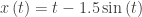
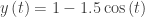
Or by the position vector with the same components $\left\langle t-1.5\sin \left( t \right),1-1.5\cos \left( t \right) \right\rangle$ .

Derivatives and the Velocity Vector

The instantaneous rate of change in the y-direction is given by dy/dt, and dx/dt gives the instantaneous rate of change in the x-direction. These are the two components of the velocity vector $\displaystyle \vec{v}\left( t \right)=\left\langle \frac{dx}{dt},\frac{dy}{dt} \right\rangle$ .

In the example, $\displaystyle \vec{v}\left( t \right) =\left\langle 1-1.5\cos \left( t \right),1.5\sin \left( t \right) \right\rangle$ . This is a vector pointing in the direction of motion and whose length, $\displaystyle \sqrt{{{\left( \frac{dx}{dt} \right)}^{2}}+{{\left( \frac{dy}{dt} \right)}^{2}}}$ , is the speed of the moving object.

In the video below the black vector is the position vector and the red vector is the velocity vector. I’ve attached the velocity vector to the tip of the position vector. Notice how the velocitiy’s length as well as its direction changes. The velocity vector pulls the object in the direction it points and there is always tangent to the path. This can be seen when the video pauses at the end and in the two figures at the end of this post.

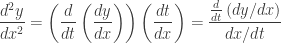
The slope of the tangent vector is the usual derivative dy/dx. It is found by differentiating dy/dt implicitly with respect to x. Therefore, $\displaystyle \frac{dy}{dx}=\frac{dy}{dt}\cdot \frac{dt}{dx}$ .

There is no need to solve for t in terms of x since dt/dx is the reciprocal of dx/dt, instead of multiplying by dt/dx we can divide by dx/dt: $\displaystyle \frac{dy}{dx}=\frac{dy/dt}{dx/dt}$ .

In the example, $\displaystyle \frac{dy}{dx}=\left( 1.5\sin \left( t \right) \right)\frac{dt}{dx}=\left( 1.5\sin \left( t \right) \right)\left( \frac{1}{1-1.5\cos \left( t \right)} \right)=\frac{1.5\sin \left( t \right)}{1-1.5\cos \left( t \right)}$

Second Derivatives and the Acceleration Vector

The components of the acceleration vector are just the derivatives of the components of the velocity vector

In the example, $\displaystyle \vec{a}\left( t \right)=\left\langle 1.5\sin \left( t \right),1.5\cos \left( t \right) \right\rangle$

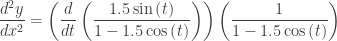
The usual second derivative $\displaystyle \frac{{{d}^{2}}y}{d{{x}^{2}}}$ is found by differentiating dy/dx, which is a function of t, implicitly with respect to x:

$\displaystyle \frac{{{d}^{2}}y}{d{{x}^{2}}}=\left( \frac{d}{dt}\left( \frac{dy}{dx} \right) \right)\left( \frac{dt}{dx} \right)=\frac{\frac{d}{dt}\left( dy/dx \right)}{dx/dt}$

In the example,

$\displaystyle \frac{{{d}^{2}}y}{d{{x}^{2}}}=\left( \frac{d}{dt}\left( \frac{1.5\sin \left( t \right)}{1-1.5\cos \left( t \right)} \right) \right)\left( \frac{1}{1-1.5\cos \left( t \right)} \right)$

$\displaystyle =\frac{\left( 1-1.5\cos \left( t \right) \right)\left( 1.5\cos \left( t \right) \right)-\left( 1.5\sin \left( t \right) \right)\left( 1.5\sin \left( t \right) \right)}{{{\left( 1-1.5\cos \left( t \right) \right)}^{2}}}\cdot \frac{1}{\left( 1-1.5\cos \left( t \right) \right)}$

$\displaystyle =\frac{1.5\cos \left( t \right)-{{1.5}^{2}}}{{{\left( 1-1.5\cos \left( t \right) \right)}^{3}}}$

The acceleration vector is the instantaneous rate of change of the velocity vector. You may think of it as pulling the velocity vector in the same way as the velocity vector pulls the moving point (the tip of the position vector). The video below shows the same situation as the first with the acceleration vectors in green attached to the tip of the velocity vector.

Here are two still figures so you can see the relationships. On the left is the starting position t = 0 with the y-axis removed for clarity. At this point the red velocity vector is $\left\langle -0.5,0 \right\rangle$ indicating that the object will start by moving directly left. The green acceleration vector is $\left\langle 0,1.5 \right\rangle$ pulling the velocity and therefore the object directly up. The second figure shows the vectors later in the first revolution. Note that the velocity vector is in the direction of motion and tangent to the path shown in blue.