Seeing Difference Quotients

Posted on August 30, 2016 by Lin McMullin

Third in the graphing calculator series.

In working up to the definition of the derivative you probably mention difference quotients. They are

The forward difference quotient (FDQ): $\displaystyle \frac{f\left( x+h \right)-f\left( x \right)}{h}$

The backwards difference quotient (BDQ): $\displaystyle \frac{f\left( x \right)-f\left( x-h \right)}{h}$ , and

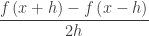
The symmetric difference quotient (SDQ): $\displaystyle \frac{f\left( x+h \right)-f\left( x-h \right)}{2h}$

Each of these is the slope of a (different) secant line and the limit of each as, if it exists, is the same and is the derivative of the function f at the point (x, f(x)). (We will assume h > 0 although this is not really necessary; if h < 0 the FDQ becomes the BDQ and vice versa.)

To see how this works you can graph a function and the three difference quotients on a graphing calculator. Here is how. Enter the function as the first function on your calculator and the difference quotients with it. Each of the difference quotients is defined in terms of Y1; this allows us to investigate the difference quotients of different functions by changing only Y1.

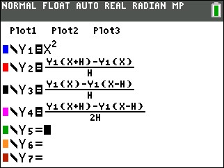
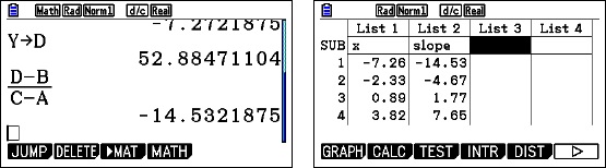
Now, on the home screen assign a value to h by typing [1] [STO] [alpha] [h]

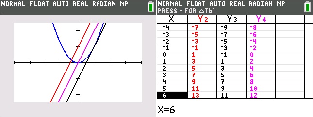
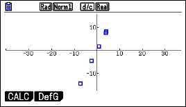
Graph the result in a square window.

The look at the table screen. (Y1 has been turned off). Can you express Y2, Y3, and Y4 in term of x?

Then change h by storing a different value, say ½, to h and graph again. Then look at the table screen again. Can you express Y2, Y3, and Y4 in term of x?

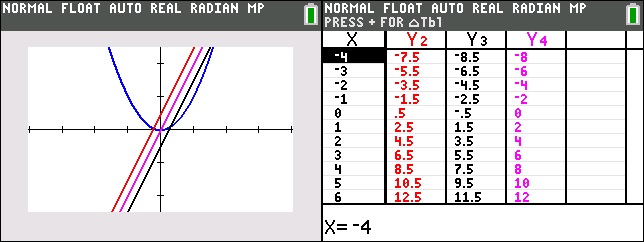
Then graph again with h = -0.1

As you can see as h gets smaller (h 0), the three difference quotients are FDQ: 2x + h, the BDQ is 2x – h, and the SDQ is 2x. They converge to the same thing. The limit of each difference quotient as h approaches zero is twice the x coordinate of the point. If you’re not sure try a smaller value of h.

The function to which each of these converge is called the derivative of the original function (Y1). In the example the derivative of x² is 2x.

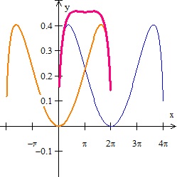
Now try another function say, Y1 = sin(x) and repeat the graphs and tables above. The tables will probably not be of much help, since the pattern is not familiar. The graph shows the function (dark blue) and only the SDQ (light blue), h = 0.1 Can you guess what the derivative might be?

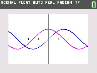
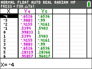
I f you guessed cos(x) you are correct. The table shows the SDQ values as Y4, and the values of cos(x) as Y5. Pretty close! If you want to get closer try h = 0.001.

If you have a CAS calculators such as the TI-Nspire or the HP PRIME you can do this activity with sliders. Also you may try this with DESMOS. Click here or on the graph below. Some interesting functions to start with are cos(x) and | x |.

And by the way, the SDQ is what most graphing calculators use to calculate the derivative. It is called nDeriv on TI calculators.

Tangent Lines

Posted on August 23, 2016 by Lin McMullin

Second in the Graphing Calculator/Technology series

This graphing calculator activity is a way to introduce the idea if the slope of the tangent line as the limit of the slope of a secant line. In it, students will write the equation of a secant line through two very close points. They will then compare their results in several ways.

Begin by having the students graph a very simple curve such as y = x² in the standard window of their calculator. Then TRACE to a point. Students will go to different points, some to the left and some to the right of the origin. ZOOM IN several times on this point until their graph appears linear (discuss local linearity here). To be sure they are on the graph push TRACE again. The coordinates of their point will be at the bottom of the screen; call this point (a, b). Return to the home screen and store the values to A and B (click here for instructions on storing and recalling numbers).

Return to the graph and push TRACE again to be sure the cursor is on the graph. Move the TRACE cursor one or two pixels away from the first point in either direction. This new point is (c, d). Return to the home screen and store the coordinates to C and D.

Enter the equation of the line through the two points on the equation entry screen in terms of A, B, C, and D. Zoom Out several times until you have returned to the original window..

Exploration 1: Have students compare and contrast their graphs with several other students and discuss their observations. (Expected observations: the lines appear tangent at each students’ original point)

Exploration 2: Ask student to compute the slope of the line through their points, again using A, B, C, and D. Collect each student’s x-coordinate, A, and their slope and enter them in list is your calculator so that they can be projected.

Study the two lists and discuss the relation is any. (Expected observations: the slope is twice the x-coordinate.) Can you write an equation of these pairs? (Expected result: y = 2x)

Finally, plot the points on the calculator using a square window. Do the points seem to lie on the line y =2x?

Extensions:

Try the same activity with other functions such as y = (1/3)x³, y = x³, or y = x⁴. Anything more difficult will still result in a tangent line, but the numerical relationship between x and the slope will probably be too difficult to see. You may also consider y = sin(x) or y = cos(x). Again, the numerical work in Exploration 2, will be too difficult to see, but on graphing the points the result may be obvious. For y = sin(x), return to the list and add a column with the cosines of the x-values. Compare these with the slopes.

Good Question 9

Posted on February 14, 2016 by Lin McMullin

This is a good question that leads to other good questions, both mathematical and philosophical. A few days ago this question was posted on a private Facebook page for AP Calculus Readers. The problem and illustration were photographed from an un-cited textbook.

Player 1 runs to first base [from home plate] at a speed of 20 ft/s while player 2 runs from second base to third base a speed of 15 ft/s. Let s be the distance between the two players. How fast is s changing when player 1 is 30 feet from home plate and Player 2 is 60 feet from second base. [A figure was given showing that the distance between the bases is 90 feet.]

Some commenters indicated some possible inconsistencies in the question, such as assuming the Player 2 is on second base when Player 1 leaves home plate. In this case the numbers don’t make sense. So, someone suggested this must be a hit-and-run situation. To which someone else replied that with a lead of that much it’s really a stolen base situation. So, the first thing to be learned here is that even writing a simple problem like this you need to take some of the real aspects into consideration. But this doesn’t change the mathematical aspects of the problem.

One of the things I noticed before I attempted to work out the solution was that Player 2 is the same distance from third base as Player 1 is from home plate. I verbalized this as “players are directly across the field from each other.” I filed this away since it didn’t seem to matter much. Wrong!

Then I worked on the problem two ways. These are shown in the appendix at the end of this post. I discovered (twice) that s’ = 0; at the moment suggested in the question the distance is not changing.

Then it hit me. Doh! – I didn’t have to do all that. So, I posted this solution (which I now notice someone beat me to):

At the time described, the players are directly across the field from each other (90 feet apart). This is the closest they come. The distance between them has been decreasing and now starts to increase. So, at this instant s is not changing (s‘ = 0).

The Philosophical Question

Then the original poster asked for someone “to post [actual] work done in calculus” and “to see some related rates.” So, I posted some “calculus” and got to thinking – the philosophical question – isn’t my first answer calculus?

I think it is. It makes use of an important calculus concept, namely that as things change, at the minimum place, the derivative is zero. Furthermore, the justification (that the distance changes from decreasing to increasing at the minimum implies the derivative is zero) is included. * Why do you need variables?

Also, this solution is approached as an extreme value (max/min) problem rather than a related rate problem. This shows a nice connection between the two types of problems.

The Related (but not related rate) Good Question

So here is another calculus question with none of the numbers we’ve grown to expect:

Two cars travel on parallel roads. The roads are w feet apart. At what rate does the distance between the cars change when the cars are w feet apart?

Notice:

That the cars could be travelling in the same or opposite directions.
Their speeds are not given.
You don’t know when or where they started; only that at some time they are opposite each other (w feet apart).
In fact, they could start opposite each other and travel in the same direction at the same speed, remaining always w feet apart.
One car could be standing still and the other just passes it.

But you can still answer the question.

(*Continuity and differentiability are given (or at least implied) in the original statement of the problem.)

Appendix

My first attempt was to set up a coordinate system with the origin at third base as shown below.

Then, taking the time indicated in the problem as t = 0, the position of Player 1 is (90, 30 + 20t) and the position of player 2 is (0, 30 – 15t). Then the distance between them is

$s=\sqrt{{{90}^{2}}+{{\left( 30-15t-\left( 30+20t \right) \right)}^{2}}}=\sqrt{{{90}^{2}}+{{\left( -35t \right)}^{2}}}$

and then

$\displaystyle {s}'\left( t \right)=\frac{2\left( -35t \right)\left( -35 \right)}{2s}\text{ and }{s}'\left( 0 \right)=0$

This is correct, but for some reason I was suspicious probably because zeros can hide things. So I re-stated this time taking t = 0 to be one second before the situation described in the problem. Now player 1’s position is (90, 10+20t) and player 2’s position is (0, 45-15t).

$s\left( t \right)=\sqrt{{{90}^{2}}+{{\left( 45-15t-\left( 10+20t \right) \right)}^{2}}}=\sqrt{{{90}^{2}}+{{\left( 30-35t \right)}^{2}}}$

$\displaystyle {s}'\left( t \right)=\frac{2\left( 35-35t \right)\left( -35 \right)}{2s}\text{ and }{s}'\left( 1 \right)=0$

____________________________________________

Determining the Indeterminate 2

Posted on December 6, 2015 by Lin McMullin

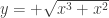
The other day someone asked me a question about the implicit relation ${{x}^{3}}-{{y}^{2}}+{{x}^{2}}=0$ . They had been asked to find where the tangent line to this relation is vertical. They began by finding the derivative using implicit differentiation:

$3{{x}^{2}}-2y\frac{dy}{dx}+2x=0$

$\displaystyle \frac{dy}{dx}=\frac{3{{x}^{2}}+2x}{2y}$

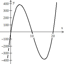
The derivative will be undefined when its denominator is zero. Substituting y = 0 this into the original equation gives ${{x}^{3}}-0+{{x}^{2}}=0$ . This is true when x = –1 or when x = 0. They reasoned that there will be a vertical tangent when x = –1 (correct) and when x = 0 (not so much). They quite wisely looked at the graph.

${{x}^{3}}-{{y}^{2}}+{{x}^{2}}=0$

The graph appears to run from the first quadrant, through the origin into the third quadrant, up to the second quadrant with a vertical tangent at x = –1, and then through the origin again and down into the fourth quadrant. It looks like a string looped over itself.

What’s going on at the origin? Where is the vertical tangent at the origin?

The short answer is that vertical tangents occur when the denominator of the derivative is zero and the numerator is not zero. When x = 0 and y = 0 the derivative is an indeterminate form 0/0.

In this kind of situation an indeterminate form does not mean that the expression is infinite, rather it means that some other way must be used to find its value. L’Hôpital’s Rule comes to mind, but the expression you get results in another 0/0 form and is no help (try it!).

My thought was to solve for y and see if that helps:

$y=\pm \sqrt{{{x}^{3}}+{{x}^{2}}}$

The graph consists of two parts symmetric to the x-axis, in the same way a circle consists of two symmetric parts above and below the x-axis. The figure below shows the top half.

$y=+\sqrt{{{x}^{3}}+{{x}^{2}}}$

So, the graph does not run from the first quadrant to the third; rather, at the origin it “bounces” up into the second quadrant. The lower half is congruent and is the reflection of this graph in the x-axis.

So, what happens at the origin and why?

The derivative of the top half is $\displaystyle \frac{dy}{dx}=\frac{3{{x}^{2}}+2x}{2\sqrt{{{x}^{3}}+{{x}^{2}}}}$ . Notice that this is the same as the implicit derivative above. Now a little simplifying; okay a lot of simplifying – who says simplifying isn’t that big a deal?

$\displaystyle \frac{dy}{dx}=\frac{x\left( 3x+2 \right)}{2\sqrt{{{x}^{2}}\left( x+1 \right)}}=\frac{x\left( 3x+2 \right)}{2\left| x \right|\sqrt{x+1}}=\left\{ \begin{matrix} \frac{3x+2}{2\sqrt{x+1}} & x>0 \\ -\frac{3x+2}{2\sqrt{x+1}} & x<0 \\ \end{matrix} \right.$

Now we see what’s happening. As x approaches zero from the right, the derivative approaches +1, and as x approaches zero from the left, the derivative approaches –1. This agrees with the graph. Since the derivative approaches different values from each side, the derivative does not exist at the origin – this is not the same as being infinite. (For the lower half, the signs of the derivative are reversed, due to the opposite sign of the denominator.)

The tangent lines at the origin are x = 1 on the right, and x = –1 on the left, hardly vertical.

What have we learned?

Indeterminate forms do not necessarily indicate an infinite value. An indeterminate form must be investigated further to see what you can learn about a function, relation, or graph.
Sometimes simplifying, or at least changing the form of an expression, is helpful and therefore necessary.

Extension: Using a graphing utility that allows sliders (Winplot, GeoGebra, Desmos, etc) enter $A{{x}^{3}}-B{{y}^{2}}+C{{x}^{2}}=0$ and explore the effects of the parameters on the graph.

_________________________

The Man Who Tried to Redeem the World with Logic

WALTER PITTS (1923-1969): Walter Pitts’ life passed from homeless runaway, to MIT neuroscience pioneer, to withdrawn alcoholic. (Estate of Francis Bello / Science Source)

I ran across this article that you might find interesting. It is about Walter Pitts one of the twentieth century’s most important mathematicians we, or at least I, have never heard of. It is from the February 5, 2015 of the science magazine Nautilus

November 2015

Posted on October 31, 2015 by Lin McMullin

Here is the list of “November Topics,” that is what AP classes usually consider from mid-November into December. There has been a lot of discussion about inverses this month at the AP Calculus Community. While not the most read on this blog, the series on inverses may be helpful in considering all the ins and outs of inverses.

The four featured posts on the first page are the most popular from this month. Speed with 3563 hits this year and 6157 hits since it first appear is one of the most popular overall. “Open or Closed?” is another poplar post.

Thinking ahead into December, the first posts on integration are here and will continue into December. (As I’ve mentioned I try to post a few weeks ahead of where most people are now, so you have some time to read and plan.)

October 13, 2014 Extremes without Calculus

November 2, 2012 Open or Closed?

November 5, 2012 Inverses

November 7, 2012 Writing Inverses

November 9, 2012 The Range of the Inverse

November 12, 2012 The Calculus of Inverses

November 14, 2012 Inverses Graphically and Numerically

November 16, 2012 Motion Problems: Same Thing, Different Context.

November 19, 2012 Speed

April 17, 2013 The Ubiquitous Particle Motion Question

September 16, 2014 Matching Motion

November 21, 2012 Derivatives of Exponential Functions

November 26, 2012 Integration Itinerary

November 18, 2012 Antidifferentiation

November 30, 2012 The Old Pump

Curves with Extrema?

Posted on October 19, 2015 by Lin McMullin

We spend a lot of time in calculus studying curves. We look for maximums, minimums, asymptotes, end behavior, and on and on, but what about in “real life”?

For some time, I’ve been trying to find a real situation determined or modeled by a non-trigonometric curve with more than one extreme value. I’ve not been very successful. I knew of only one and discovered a second in writing this post. Here is an example that illustrates what I mean.

Example 1: This is a very common calculus example. Squares are cut from the corners of a cardboard sheet that measures 20 inches by 40 inches. The remaining sides are folded up to make a box. How large should the squares be to make a box of the largest possible volume?

If we let x = the length of the side of the square, then the volume of the box is given by V = x (20 –2 x)(40 – 2x)

The graph of the volume is shown in Figure 1 and sure enough we have a polynomial curve that has two extreme values. But wait. Do we really have two extreme values? The domain of the equation appears to be all real numbers, but in fact it is 0 < x < 10, since x cannot be negative, and if x > 10, then the (20 –2 x) side is negative and that won’t work either. Figure 2 shows the true situation. There is only one extreme value.

: Figure 1

: Figure 2

Example 2: This is also an optimization problem, but a bit more difficult. A sector is cut from a circular paper disk of radius 1. The remaining part of the disk is formed into a cone. How long should the curved part of the sector be so that the cone has the maximum volume? You might want to try this before you read further.

Let x be the length of curved part of the sector See Figure 3.

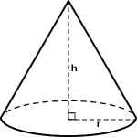
The radius of the disk becomes the slant height of the cone. The circumference of the disk is $2\pi \left( 1 \right)$ and so the circumference of the base of the cone is $C=2\pi \left( 1 \right)-x$ and its radius is $\displaystyle r=\frac{2\pi -x}{2\pi }=1-\frac{x}{2\pi }$ . The height, h of the cone is 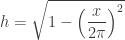$\displaystyle h=\sqrt{1-{{\left( \frac{x}{2\pi } \right)}^{2}}}$ . See figure 4.

: Figure 3

: Figure 4

The volume of the cone is . $\displaystyle V=\frac{\pi }{3}{{\left( 1-\frac{x}{2\pi } \right)}^{2}}\sqrt{{{1}^{2}}-{{\left( 1-\frac{x}{2\pi } \right)}^{2}}}$

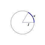
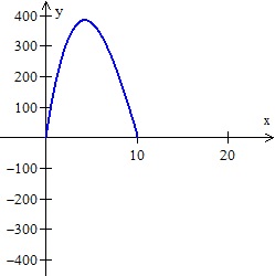
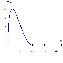
The graph of this equation is shown in Figure 5, and has two maximum values and a minimum. The domain appears to be $0<x<4\pi$ . But if $x>2\pi$ the piece you cut out will be larger than the original disk (and the expression under the radical will be negative). So our domain will be $0<x<2\pi$ (the endpoints correspond to not cutting any sector or cutting away the entire disk. The graph is shown in Figure 6 with, alas, only one extreme value.

: Figure 5

: Figure 6

(For the original expression the minimums are at $x=0,\ 2\pi ,\text{ and }4\pi$ and the maximums are at $x\approx 1.153\text{ and }x\approx 11.413$ . A CAS will help with these calculations or just use a graphing calculator.)

Extension 1: Find the value of x that will make the largest volume when the piece cut out is formed into a cone. Compare the two graphs and explain their congruence. See Figure 7.
Extension 2: Here I finally found what I was after. – a situation with more than one extreme value. Find the value of x that will make the largest total volume formed when the volume of the original cone and the cone formed by the piece cut out. Compare the first two graphs and the graph of this volume. See figure 8 – the magenta graph.

: Figure 7

: Figure 8

The Mae West Curve

There is at least one real situation that is modeled by a function with several extreme values. Spud’s blog gives the following explanation and illustration.

“When a Uranium (or Plutonium) atom fission, or splits, you end up with two much lighter atoms, called fission products, or daughter nuclides. The U-235 nucleus can split into a myriad of combinations, but some combinations are more likely than others.

“[Figure 9 below] shows the percentage of fission products by [atomic] mass[, A]. [This is] called the Mae West curve. … Note that the more likely fission products have two peaks at a mass of about 95 and 135.”

Thus we have a real life illustration of a model that has three extreme values in its domain.

The model graphed in Figure 9 is known as the “Mae West Curve,” named after Mae West (1893 – 1980) and actress, playwright and screenwriter.

: Figure 9: The “Mae West” Curve

If you know of any other real situations with more than one extreme, please let us know. Use the “comment” button below.

Good Question 7 – 2009 AB 3

Posted on October 5, 2015 by Lin McMullin

Another in my occasional series on Good Questions to teach from. This is the Mighty Cable Company question from the 2009 AB Calculus exam, number 3

This question presented students with a different situation than had been seen before. It is a pretty standard “in-out” question, except that what was going in and out was money. Students were told that the Mighty Cable Company sold its cable for $120 per meter. They were also told that the cost of the cable varied with its distance from the starting end of the cable. Specifically, the cost of producing a portion of the cable x meters from the end is $6\sqrt{x}$ dollars per meter. Profit was defined as the difference between the money the company received for selling the cable minus the cost of producing the cable.

Students had a great deal of trouble answering this question. (The mean was 1.92 out of a possible 9 points. Fully, 36.9% of students earned no point; only 0.02% earned all 9 points.) This was probably because they had difficulty in interpreting the question and translating it into the proper mathematical terms and symbols. Since economic problems are not often seen on AP Calculus exams, students needed to be able to use the clues in the stem:

The $120 per meter is a rate. This should be deduced from the units: dollars per meter.
The cost of producing the portion of cable x meters from one end cable is also a rate for the same reason. In economics this is called the marginal cost; the students did not need to know this term.
The profit is an amount that is a function of x, the length of the cable.

Part (a): Students were required to find the profit from the sale of a 25-meter cable. This is an amount. As always, when asked for an amount, integrate a rate. In this case integrate the difference between the rate at which the cable sells and the cost of producing it.

$\displaystyle P(25)=\int_{0}^{25}{\left( 120-6\sqrt{x} \right)dx}=\$2500$

$\displaystyle P(25)=120(25)-\int_{0}^{25}{6\sqrt{x}\ dx}=\$2500$

Part (b): Students were asked to explain the meaning of $\displaystyle \int_{25}^{30}{6\sqrt{x}dx}$ in the context of the problem. Since the answer is probably not immediately obvious, here is the reasoning involved.

This is the integral of a rate and therefore, gives the amount (of money) needed to manufacture the cable. This can be found by a unit analysis of the integrand: $\displaystyle \frac{\text{dollars}}{\text{meter}}\cdot \text{meters}=\text{dollars}$ .

Let C be the cost of production, so $\displaystyle \frac{dC}{dx}=6\sqrt{x}$ , and therefore, $\displaystyle \int_{25}^{30}{6\sqrt{x}dx}=C\left( 30 \right)-C\left( 25 \right)$ by the Fundamental Theorem of Calculus (FTC).

Therefore, $\displaystyle \int_{25}^{30}{6\sqrt{x}dx}$ is the difference in dollars between the cost of producing a cable 30 meters long, C(30), and the cost of producing a cable 25 meters long, C(25). (Another acceptable is that the integral is the cost in dollars of producing the last 5 meters of a 30 meter cable.)

Part (c): Students were asked to write an expression involving an integral that represents the profit on the sale of a cable k meters long.

Part (a) serves as a hint for this part of the question. Here the students should write the same expression as they wrote in (a) with the 25 replaced by k.

$\displaystyle P(k)=\int_{0}^{k}{\left( 120-6\sqrt{x} \right)dx}$

$\displaystyle P(k)=120k-\int_{0}^{k}{6\sqrt{x}\ dx}$

Part d: Students were required to find the maximum profit that can be earned by the sale of one cable and to justify their answer. Here they need to find when the rate of change of the profit (the marginal profit) changes from positive to negative.

Using the FTC to differentiate either of the answers in part (c) or by starting fresh from the given information:

$\displaystyle \frac{dP}{dx}=120-6\sqrt{x}$

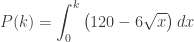
$\displaystyle \frac{dP}{dx}=0$ when x = 400 and P(400)= $16,000.

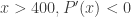Justification: The maximum profit on the sale of one cable is $16,000 for a cable 400 meters long. For $0<x<400,{P} '(x)>0$ and for $x>400,{P} '(x)<0$ therefore, the maximum profit occurs at x = 400. (The First Derivative Test).

Once students are familiar with in-out questions, this is a good question to challenge them with. The actual calculus is not that difficult or unusual but concentrating on the translation of the unfamiliar context into symbols and calculus ideas is different. Show them how to read the hints in the problem such as the units.

Steel cable or steel wire rope as it is called also has some interesting geometry in its construction. You can find many good illustrations of this, such as the ones below, by Googling “steel wire rope.”

This slideshow requires JavaScript.

Teaching Calculus

The pleasure lies not in discovering the truth, but in searching for it.

Category Archives: Derivatives

Seeing Difference Quotients

Tangent Lines

Determining the Indeterminate 2

November 2015

Curves with Extrema?

Good Question 7 – 2009 AB 3

Share this:

Share this:

Share this:

Share this:

Share this:

Share this:

Share this: