The Definite Integral and the FTC

Posted on November 17, 2017 by Lin McMullin

The Definition of the Definite Integral.

The definition of the definite integrals is: If f is a function continuous on the closed interval [a, b], and $a={{x}_{0}}<{{x}_{1}}<{{x}_{2}}<\cdots <{{x}_{{n-1}}}<{{x}_{n}}=b$ is a partition of that interval, and $x_{i}^{*}\in [{{x}_{{i-1}}},{{x}_{i}}]$ , then

$\displaystyle \underset{{\left| {\left| {\Delta x} \right|} \right|\to 0}}{\mathop{{\lim }}}\,\sum\limits_{{i=0}}^{n}{{f\left( {x_{i}^{*}} \right)}}\left( {{{x}_{i}}-{{x}_{{i-i}}}} \right)=\int\limits_{a}^{b}{{f\left( x \right)dx}}$

The left side of the definition is, of course, any Riemann sum for the function f on the interval [a, b]. In addition to being shorter, the right side also tells you about the interval on which the definite integral is computed. The expression $\left\| {\Delta x} \right\|$ is called the “norm of the partition” and is the longest subinterval in the partition. Usually, all the subintervals are the same length, $\frac{{b-a}}{n}$ , and this is the last you will hear of the norm. With all the subdivisions of the same length this can be written as

$\displaystyle \underset{{n\to \infty }}{\mathop{{\lim }}}\,\sum\limits_{{i=0}}^{n}{{f\left( {x_{i}^{*}} \right)}}\frac{{b-a}}{n}=\int\limits_{a}^{b}{{f\left( x \right)dx}}$

Other than that, there is not much more to the definition. It is simply a quicker and more efficient notation for the sum.

The Fundamental Theorem of Calculus (FTC).

First recall the Mean Value Theorem (MVT) which says: If a function is continuous on the closed interval [a, b] and differentiable on the open interval (a, b) then there exist a number, c, in the open interval (a, b) such that ${f}'\left( c \right)\left( {b-a} \right)=f\left( b \right)-f\left( a \right)$ .

Next, let’s rewrite the definition above with a few changes. The reason for this will become clear.

$\int\limits_{a}^{b}{{{f}'\left( x \right)dx}}=\underset{{\left| {\left| {\Delta x} \right|} \right|\to 0}}{\mathop{{\lim }}}\,\sum\limits_{{i=0}}^{n}{{{f}'\left( {{{c}_{i}}} \right)\left( {{{x}_{i}}-{{x}_{{i-i}}}} \right)}}$

Since every function is the derivative of another function (even though we may not know that function or be able to write a closed-form expression for it), I’ve expressed the function as a derivative, I’ve also chosen the point in each subinterval, ${{c}_{i}}$ , to be the number in each subinterval guaranteed by the MVT for that subinterval.

Then, $\displaystyle {f}'\left( {{{c}_{i}}} \right)\left( {{{x}_{i}}-{{x}_{{i-i}}}} \right)=f\left( {{{x}_{i}}} \right)-f\left( {{{x}_{{i-1}}}} \right)$ . Making this substitution, we have

$\int\limits_{a}^{b}{{{f}'\left( x \right)dx}}=\underset{{\left| {\left| {\Delta x} \right|} \right|\to 0}}{\mathop{{\lim }}}\,\sum\limits_{{i=0}}^{n}{{\left( {f\left( {{{x}_{i}}} \right)-f\left( {{{x}_{{i-1}}}} \right)} \right)}}$

$\displaystyle =f\left( {{{x}_{1}}} \right)-f\left( {{{x}_{0}}} \right)+f\left( {{{x}_{2}}} \right)-f\left( {{{x}_{1}}} \right)+f\left( {{{x}_{3}}} \right)-f\left( {{{x}_{2}}} \right)+\cdots +f\left( {{{x}_{n}}} \right)-f\left( {{{x}_{{n-1}}}} \right)$

$\displaystyle =f\left( {{{n}_{n}}} \right)-f\left( {{{x}_{0}}} \right)$

And since ${{x}_{0}}=a$ and ${{x}_{n}}=b$ ,

$\displaystyle \int_{a}^{b}{{{f}'\left( x \right)dx}}=f\left( b \right)-f\left( a \right)$

This equation is called the Fundamental Theorem of Calculus. In words, it says that the integral of a function can be found by evaluating the function of which the integrand is the derivative at the endpoints of the interval and subtracting the values. This is a number that may be positive, negative, or zero depending on the function and the interval. The function of which the integrand is the derivative, is called the antiderivative of the integrand.

The real meaning and use of the FTC is twofold:

It says that the integral of a rate of change (i.e. a derivative) is the net amount of change. Thus, when you want to find the amount of change – and you will want to do this with every application of the derivative – integrate the rate of change.
It also gives us an easy way to evaluate a Riemann sum without going to all the trouble that is necessary with a Riemann sum; simply evaluate the antiderivative at the endpoints and subtract.

At this point I suggest two quick questions to emphasize the second point:

Find $\int_{3}^{7}{{2xdx}}$ .

Ask if anyone knows a function whose derivative is 2x? Your students will know this one. The answer is x², so

$\displaystyle \int_{3}^{7}{{2xdx}}={{7}^{2}}-{{3}^{2}}=40$ .

Much easier than setting up and evaluating a Riemann sum!

2. Then ask your students to find the area enclosed by the coordinate axes and the graph of cos(x) from zero to $\frac{\pi }{2}$ . With a little help they should arrive at

$\displaystyle \int_{0}^{{\pi /2}}{{\cos \left( x \right)dx}}$ .

Then ask if anyone knows a function whose derivative is cos(x). it’s sin(x), so

$\displaystyle \int_{0}^{{\pi /2}}{{\cos \left( x \right)dx}}=\sin \left( {\frac{\pi }{2}} \right)-\sin \left( 0 \right)=1-0=1$ .

At this point they should be convinced that the FTC is a good thing to know.

There is another form of the FTC that is discussed in More About the FTC.

Table & Riemann Sum Questions (Type 5)

Posted on March 17, 2017 by Lin McMullin

Tables may be used to test a variety of ideas in calculus including analysis of functions, accumulation, position-velocity-acceleration, theory and theorems among others. Numbers and working with numbers is part of the Rule of Four and table problems are one way this is tested.

What students should be able to do:

Find the average rate of change over an interval
Approximate the derivative using a difference quotient. Use the two values closest to the number at which you are approximating. This amounts to finding the slope. Show the quotient even if you can do the arithmetic in your head.
Use Riemann sums (left, right, midpoint), or a trapezoidal approximation to approximate the value of a definite integral using values in the table (typically with uneven subintervals). The Trapezoidal Rule, per se, is not required; it is expected that students will add the areas of a small number of trapezoids without reference to a formula.
Average value, average rate of change, Rolle’s theorem, the Mean Value Theorem and the Intermediate Value Theorem. (See 2007 AB 3 – four simple parts that could be multiple-choice questions; the mean on this question was 0.96 out of a possible 9.)
These questions are usually presented in some context and answers should be in that context.
Unit analysis.

Do’s and Don’ts

Do: Remember that you do not know what happens between the values in the table unless some other information is given. For example, don’t assume that the largest number in the table is the maximum value of the function.

Do: Show what you are doing even if you can do it in your head. If you’re finding a slope, show the quotient.

Do Not do arithmetic: A long expression consisting entire of numbers such as you get when doing a Riemann sum, does not need to be simplified in any way. If you simplify correct answer incorrectly, you will lose credit. However, do not leave expression such as R(3) – pull its numerical value from the table.

Do Not: Find a regression equation and then use that to answer parts of the question. While regression is perfectly good mathematics, regression equations are not one of the four things students may do with their calculator. Regression gives only an approximation of our function. The exam is testing whether students can work with numbers.

Shorter questions on this concept appear in the multiple-choice sections. As always, look over as many questions of this kind from past exams as you can find.

Tuesday Match 21: Differential Equations (Type 6)

Friday March 24: Others (Type 7: related rates, implicit differentiation, etc.)

Tuesday March 28: for BC Parametric Equation (Type 8)

Good Question 11 – Riemann Reversed

Posted on November 29, 2016 by Lin McMullin

Good Question 11 – or not.

The question below appears in the 2016 Course and Exam Description (CED) for AP Calculus (CED, p. 54), and has caused some questions since it is not something included in most textbooks and has not appeared on recent exams. The question gives a Riemann sum and asks for the definite integral that is its limit. Another example appears in the 2016 “Practice Exam” available at your audit website; see question AB 30. This type of question asks the student to relate a definite integral to the limit of its Riemann sum. These are called reversal questions since you must work in reverse of the usual order. Since this type of question appears in both the CED examples and the practice exam, the chances of it appearing on future exams look good.

To the best of my recollection the last time a question of this type appeared on the AP Calculus exams was in 1997, when only about 7% of the students taking the exam got it correct. Considering that by random guessing about 20% should have gotten it correct, this was a difficult question. This question, the “radical 50” question, is at the end of this post.

Example 1

Which of the following integral expressions is equal to $\displaystyle \underset{n\to \infty }{\mathop{\lim }}\,\sum\limits_{k=1}^{n}{\left( \sqrt{1+\frac{3k}{n}}\cdot \frac{1}{n} \right)}$ ?

There were 4 answer choices that we will consider in a minute.

The first key to answering the question is to recognize the limit as a Riemann sum. In general, a right-side Riemann sum for the function f on the interval [a, b] with n equal subdivisions, has the form:

$\displaystyle \underset{n\to \infty }{\mathop{\lim }}\,\sum\limits_{k=1}^{n}{\left( f\left( a+\frac{b-a}{n}\cdot k \right)\cdot \frac{b-a}{n} \right)}=\int_{a}^{b}{f\left( x \right)dx}$

To evaluate the limit and express it as an integral, we must identify, a, b, and f. I usually begin by looking for $\displaystyle \frac{b-a}{n}$ . Here $\displaystyle \frac{b-a}{n}=\frac{1}{n}$ and from this conclude that b – a = 1, so b = a + 1.

Usually, you can start by considering a = 0 , which means that the $\displaystyle \frac{b-a}{n}\cdot k$ becomes the “x.”. Then rewriting the radicand as $\displaystyle 1+3\frac{1}{n}k=1+3\left( a+\frac{1}{n}\cdot k \right)$ , it appears the function is $\sqrt{1+3x}$ and the limit is $\displaystyle \int_{0}^{1}{\sqrt{1+3x}}dx=\frac{14}{9}$ .

The answer choices are

(A) $\displaystyle \int_{0}^{1}{\sqrt{1+3x}}dx$ (B) $\displaystyle \int_{0}^{3}{\sqrt{1+x}}dx$ (C) $\displaystyle \int_{1}^{4}{\sqrt{x}}dx$ (D) $\displaystyle \tfrac{1}{3}\int_{0}^{3}{\sqrt{x}}dx$

The correct choice is (A), but notice that choices B, C, and D can be eliminated as soon as we determine that b = a + 1. That is not always the case.

Let’s consider another example:

Example 2: $\displaystyle \underset{n\to \infty }{\mathop{\lim }}\,\sum\limits_{k=1}^{n}{\left( {{\left( 2+\frac{3}{n}k \right)}^{2}}\left( \frac{3}{n} \right) \right)}=$

As before consider $\displaystyle \frac{b-a}{n}=\frac{3}{n}$ , which implies that b = a + 3. With a = 0, the function appears to be ${{\left( 2+x \right)}^{2}}$ on the interval [0, 3], so the limit is $\displaystyle \int_{0}^{3}{{{\left( 2+x \right)}^{2}}}dx=39$

BUT

What if we take a = 2? If so, the limit is $\displaystyle \int_{2}^{5}{{{x}^{2}}dx}=39$ .

And now one of the “problems” with this kind of question appears: the answer written as a definite integral is not unique!

Not only are there two answers, but there are many more possible answers. These two answers are horizontal translations of each other, and many other translations are possible, such as $\displaystyle \int_{-25.65}^{-22.65}{{{\left( 27.65+x \right)}^{2}}dx}=39$ .

The same thing can occur in other ways. Returning to example 1,and using something like a u-substitution, we can rewrite the original limit as $\displaystyle \frac{1}{3}\cdot \underset{n\to \infty }{\mathop{\lim }}\,\sum\limits_{k=1}^{n}{\left( \sqrt{1+\frac{3k}{n}}\cdot \frac{3}{n} \right)}$ .

Now b = a + 3 and the limit could be either $\displaystyle \frac{1}{3}\int_{0}^{3}{\sqrt{1+x}}dx=\frac{14}{9}$ or $\displaystyle \frac{1}{3}\int_{1}^{4}{\sqrt{x}}dx=\frac{14}{9}$ , among others.

My opinions about this kind of question.

The real problem with the answer choices to Example 1 is that they force the student to do the question in a way that gets one of the answers. It is perfectly reasonable for the student to approach the problem a different way, and get a different correct answer that is not among the choices. This is not good.

The problem could be fixed by giving the answer choices as numbers. These are the numerical values of the 4 choices:(A) 14/9 (B) 14/3 (C) 14/3 (D) $2\sqrt{3}/3$ . As you can see that presents another problem. Distractors (wrong answers) are made by making predictable calculus mistakes. Apparently, two predictable mistakes give the same numerical answer; therefore, one of them must go.

A related problem is this: The limit of a Riemann sum is a number; a definite integral is a number. Therefore, any definite integral, even one totally unrelated to the Riemann sum, which has the correct numerical value, is a correct answer.

I’m not sure if this type of question has any practical or real-world use. Certainly, setting up a Riemann sum is important and necessary to solve a variety of problems. After all, behind every definite integral there is a Riemann sum. But starting with a Riemann sum and finding the function and interval does not seem to me to be of practical use.

The CED references this question to MPAC 1: Reasoning with definitions and theorems, and to MPAC 5: Building notational fluency. They are appropriate,and the questions do make students unpack the notation.

My opinions notwithstanding, it appears that future exams will include questions like these.

These questions are easy enough to make up. You will probably have your students write Riemann sums with a small value of n when you are teaching Riemann sums leading up to the Fundamental Theorem of Calculus. You can make up problems like these by stopping after you get to the limit, giving your students just the limit, and having them work backwards to identify the function(s) and interval(s). You could also give them an integral and ask for the associated Riemann sum. Question writers call questions like these reversal questions since the work is done in reverse of the usual way.

Here is the question from 1997, for you to try. The answer is below.

Answer B. Hint n = 50

Revised 5-5-2022

Good Question 8 – or not?

Posted on January 5, 2016 by Lin McMullin

Today’s question is not a good question. It’s a bad question.

But sometimes a bad question can become a good one.

This one leads first to a discussion of units, then to all sorts of calculus.

Here’s the question a teacher sent me this week taken from his textbook:

The normal monthly rainfall at the Seattle-Tacoma airport can be approximated by the model $R=3.121+2.399\sin \left( 0.524t+1.377 \right)$ , where R is measured in inches and t is the time in months, t = 1 being January. Use integration to approximate the normal annual rainfall. Hint: Integrate over the interval [0,12].

Of course, with the hint it’s not difficult to know what to do and that makes it less than a good question right there. The answer is $\displaystyle \int_{0}^{12}{R(t)dt=37.4736}$ inches. You could quit here and go on to the next question, but …

Then a student asked. “If R is in inches shouldn’t be in units of the integral be inch-months, since the unit of an integral is the unit of the integrand times the units of the independent variable?” Well, yes, they should. So, what’s up with that?

Also, the teacher figured that the integral of a rate is an amount and our answer is an amount, so why isn’t the integrand a rate?

The only answer I could come up with is that the statement “R is measured in inches” is incorrect; R should be measured in inches /month. The opening phrase “normal monthly rainfall” also seems to point to the correct units for R being inches/month.

Problem solved; or maybe does this lead to a different concern?

The teacher pointed out that R(6) = 0.7658 inches is a reasonable answer for the amount of rain in June whereas $\displaystyle \int_{0}^{6}{R(t)dt=}20.4786$ is not.

If R is a rate, then the amount of rain that falls in June (t = 6) is given by $\displaystyle \int_{5}^{6}{R(t)dt}=0.9890$ .

From here on we will assume that R is a rate with units of inches/month. Here are the individual monthly rates calculated with a CAS.

The total amount of rainfall (second line above) appears be R(1) + R(2) + R(3) + … +R(12) = 37.4742. This is very close to the amount calculated by integration.

The slight difference of 0.0006 is not a round off error.

Remember, behind every definite integral there is a Riemann sum!

Again, the units are the problem. Why does the sum of the monthly rates seem to give the total amount? The reason is that the terms of the sequence above are actually the values of a right-side Riemann sum of the rate, R(t), over the interval [0,12] with 12 equal subdivisions of width 1 (month) each with the 1’s left out as 1’s often are. Therefore, their sum should come close to the total yearly rainfall, but it is really just an approximation of it.

The actual total for any month, n, is given by $\displaystyle \int_{n-1}^{n}{r(t)}dt$ . For example the amount of rain that falls in June is given by $\displaystyle \int_{5}^{6}{R(t)dt}=0.9890$ inches.

Here is the sequence of the actual monthly rainfall values in inches, and their sum.

This agrees with the integral. Why? Because one of the properties of integrals tell us that $\displaystyle \sum\limits_{n=1}^{12}{\int_{n-1}^{n}{r(t)dt}}=\int_{0}^{12}{r(t)dt}$ .

Another instructive thing with this integral is this: The function $R=3.121+2.399\sin \left( 0.524t+1.377 \right)$ is periodic with a period of $\frac{2\pi }{0.524}\approx 11.9908\approx 12$ . So the sine function takes on (almost) all its values in a year, as you would expect. Since the sine values all but cancel each other out

$\displaystyle \int_{0}^{12}{3.121+2.399\sin \left( 0.524t+1.377 \right)dt}\approx \int_{0}^{12}{3.121dt=3.121\left( 12-0 \right)=37.452}$ . Close!

The total rainfall divided by 12 is $\frac{37.452}{12}=3.121$ this must be close to the average rainfall each month. The average rainfall is $\displaystyle \frac{1}{12}\int_{0}^{12}{R\left( t \right)dt}=3.1228$ inches. Close, again!

So, there you have it. Is this a good question or not? We considered all these concepts while working not just with an equation but with numbers from a poorly stated problem:

Reading and interpreting words.
Unit analysis
Integration by technology
Realizing that a pretty good approximation is not correct, due again to units.
A Riemann sum approximation in a real situation that comes very close to the value by integration
Using a property of a periodic function to greatly simplify an integral
Finding average value two ways

So, it turned out to be a sunny day in Seattle.

Foreshadowing the FTC

Posted on December 15, 2014 by Lin McMullin

This is an example to help prepare students to tackle the Fundamental Theorem of Calculus (FTC). Use it after the lesson on Riemann sums and the definition of the definite integral, but before the FTC derivation.

Consider the area, A, between the graph of $f\left( x \right)=\cos \left( x \right)$ and the x-axis on the interval $\left[ 0,\tfrac{\pi }{2} \right]$ . Set up a Riemann sum using the general partition:

$0={{x}_{0}}<{{x}_{1}}<{{x}_{2}}<{{x}_{3}}<\cdots <{{x}_{n-2}}<{{x}_{n-1}}<{{x}_{n}}=\tfrac{\pi }{2}$

$\displaystyle A=\int_{0}^{{\scriptstyle{}^{\pi }\!\!\diagup\!\!{}_{2}\;}}{\cos \left( x \right)dx}=\underset{\Delta x\to 0}{\mathop{\lim }}\,\sum\limits_{i=1}^{n}{\cos \left( {{c}_{i}} \right)\left( {{x}_{i}}-{{x}_{i-1}} \right)}$

Since we can choose the value of ${{c}_{i}}$ any way we want, let’s take the same intervals and use ${{c}_{i}}$ the number guaranteed by the Mean Value Theorem for the function $F\left( x \right)=\sin \left( x \right)$ on the each sub-interval interval. That is, on each sub-interval at $x={{c}_{i}}$

$\left. \frac{d}{dx}\sin \left( x \right) \right|_{x={{c}_{i}}}^{{}}=\cos \left( {{c}_{i}} \right)=\frac{\sin \left( {{x}_{i}} \right)-\sin \left( {{x}_{i-1}} \right)}{\left( {{x}_{i}}-{{x}_{i-1}} \right)}$

Then, substituting into the Riemann sum above

$\displaystyle A=\underset{\Delta x\to 0}{\mathop{\lim }}\,\sum\limits_{i=1}^{n}{\cos \left( {{c}_{i}} \right)\left( {{x}_{i}}-{{x}_{i-1}} \right)}=\underset{\Delta x\to 0}{\mathop{\lim }}\,\sum\limits_{i=1}^{n}{\frac{\sin \left( {{x}_{i}} \right)-\sin \left( {{x}_{i-1}} \right)}{\left( {{x}_{i}}-{{x}_{i-1}} \right)}\left( {{x}_{i}}-{{x}_{i-1}} \right)}$

$\displaystyle A=\underset{\Delta x\to 0}{\mathop{\lim }}\,\sum\limits_{i=1}^{n}{\left( \sin \left( {{x}_{i}} \right)-\sin \left( {{x}_{i-1}} \right) \right)}$

Now writing out the terms we have a telescoping series:

$\displaystyle A=\left( \sin \left( {{x}_{1}} \right)-\sin \left( {{x}_{0}} \right) \right)+\left( \sin \left( {{x}_{2}} \right)-\sin \left( {{x}_{1}} \right) \right)+\left( \sin \left( {{x}_{3}} \right)-\sin \left( {{x}_{2}} \right) \right)+$

$\displaystyle \cdots +\left( \sin \left( {{x}_{n-1}} \right)-\sin \left( {{x}_{n-2}} \right) \right)+\left( \sin \left( {{x}_{n}} \right)-\sin \left( {{x}_{n-1}} \right) \right)$

$\displaystyle A=\sin \left( {{x}_{n}} \right)-\sin \left( {{x}_{0}} \right)$

$\displaystyle A=\sin \left( \tfrac{\pi }{2} \right)-\sin \left( 0 \right)=1$

As you can see, this is really just the derivation of the FTC applied to a particular function. Now the students should have a better idea of what’s going on when you solve the problem in general, i.e. when you prove the FTC.

Variations on a Theme – 2

Posted on June 28, 2013 by Lin McMullin

This is the second in an occasional series on adapting and expanding AP calculus exam questions. Variations on multiple-choice questions may make other multiple-choice questions, or, if you do not like making up all the “wrong” choices they can be changed to short answer questions for use in your class homework or test. Other variations make for good discussion questions.

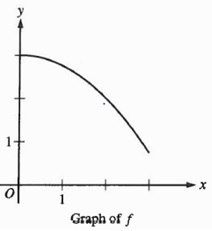
Today we will take a look at 2008 AB 10. This question gave the graph below and asked which of $\displaystyle \int_{1}^{3}{f\left( x \right)dx}$ , a left, right, or midpoint Riemann sum approximation, or a trapezoidal sum approximation of the integral all with four subintervals of equal length has the least value.

I’ll refer to these as I, L, R, M and T. The answer is R as a quick sketch will show.

In the discussion we will assume the curve does not change direction or concavity over the interval of integration. The answers to the questions in the variations are at the end of this post.

Variation 1: The question seems pretty easy so let’s beef it up a bit. How about asking the student to put I, L, R, M and T in order from smallest to largest? For a multiple-choice question answer choices are inequalities with all 5 sums in them.

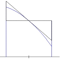
The midpoint Riemann sum may be the most difficult to see. Here is the way to explain it. See the figure below.

On each subinterval draw the horizontal segment at the function value at the midpoint of the interval. At this same point draw a tangent segment from one side of the interval to the other. This forms two congruent triangles with the horizontal segment and the edges of the interval.

Therefore, this midpoint trapezoid and the midpoint rectangle have the same area. Then because of the concavity, we see that in this case the midpoint Riemann sum, M, will be larger than the integral, I. With the same concavity the trapezoidal approximation will lie below the curve and therefore T < I < M. This will be true for any curve that is concave down. The opposite is true for a curve that is concave up: M < I < T. M and T are always on opposite sides of I.

Variation 2: Change the number of subintervals, but keep the same number for each sum. Does this change anything?

Variation 3: Change the number of subintervals so that the sums over the same interval have a different number of subintervals. Does this change anything?

Variation 4: Change the shape of the curve to one of the other 4 shapes that a curve may have. How does this change the order of the sums?

Variation 5: Move the graph from above the x-axis to below. Does this change anything?

Variation 6: The reversal problem. Suppose that L < T < I < M < R; describe the shape of the curve. Other orders can be used as well. In fact this idea has appeared on an AP calculus exams. In 2003 AB 85 students were told that a trapezoidal sum over approximates and a right Riemann sum under approximates a certain integral. The question asked which of 5 graphs could be the graph of the function.

___________________

If you have other variations please click “Leave a Comment” to share them. If you have variations on a different question please share them as well.

___________________

Answers:

Variation 1: R < T < I < M < L

Variation 2: No. Since the order will be the same on each subinterval adding them will not change the order.

Variation 3: This makes a difference. In the first figure above, consider a trapezoidal sum with one subinterval compared to a right Riemann sum with many subintervals. The right Riemann sum will be very close to the integral with its rectangles ending above the trapezoidal segment between the endpoints. In this case T < R for the figure shown.

Variation 4: The left and right Riemann sums depend on whether the curve is decreasing or increasing. The Trapezoidal sum and the midpoint Riemann sum depend on the concavity. For example, an increasing concave up curve the order is L < M < I < T < R.

Variation 5: No. If the curve is entirely below the x-axis all the values will be negative, but all the results discussed in the other variations will be the same; the order will not change.

Variation 6: The curve is increasing and concave down.

Area Between Curves

Posted on January 7, 2013 by Lin McMullin

Applications of Integration 1 – Area Between Curves

The first thing to keep in mind when teaching the applications of integration is Riemann sums. The thing is that when you set up and solve the majority of application problems you cannot help but develop a formula for the situation. Students think formulas are handy and go about memorizing them badly. By which I mean they forget or never learn where the various things in the formula come from. A slight change in the situation and they are lost. Behind every definite integral stands a Riemann sum; each application should be approached through its Riemann sum. If students understand that, they will make fewer mistakes with the “formula.”

As I suggested in a previous post, I believe all area problems should be treated as the area between two curves. If you build the Riemann sum rectangle between the graph and the axis and calculate its vertical side as the upper function minus the lower (or right minus left if you use horizontal rectangles) you will always get the correct integral for the area. If the upper curve is the x-axis, then the vertical sides of the Riemann sums are (0 – f(x)) and you get a positive area as you should.

If both your curves are above the x-axis, then it is tempting to explain what you are doing as subtracting the area between the lower curve and the x-axis from the area between the upper curve and the x-axis. And this is not wrong. It just does not work very smoothly when one, both or parts of either are below the x-axis. Then you go into all kinds of contortions explaining things in terms of positive and negative areas. Why go there?

Regardless of where the two curves are relative to the x-axis, the vertical distance between them is the upper value minus the lower, f(x) – g(x). It does not matter if one or both functions are negative on all or part of the interval, the difference is positive and the area between them is

$\displaystyle \underset{n\to \infty }{\mathop{\lim }}\,\sum\limits_{i=1}^{n}{\left( f\left( {{x}_{i}} \right)-g\left( {{x}_{i}} \right) \right)\Delta {{x}_{i}}}=\int_{a}^{b}{f\left( x \right)-g\left( x \right)dx}$ .

Furthermore, this Riemann sum rectangle is used in other applications. It is the one rotated in both the washer and shell method of finding volumes. So in area and all applications be sure your students don’t just memorize formulas, but keep their eyes on the rectangle and the Riemann sum.

Finally, if the graphs cross in the interval so that the upper and lower curves change place, you may (1) either break the problem into several pieces so that your integrands are always of the form upper minus lower, or (2) if you intend to do the computation using technology, set up the integral as

$\displaystyle \int_{a}^{b}{\left| f\left( x \right)-g\left( x \right) \right|dx}$ .

Teaching Calculus

The pleasure lies not in discovering the truth, but in searching for it.

Tag Archives: Riemann sum

The Definite Integral and the FTC

Table & Riemann Sum Questions (Type 5)

Good Question 11 – Riemann Reversed

Good Question 8 – or not?

Foreshadowing the FTC

Variations on a Theme – 2

Area Between Curves

Share this:

Share this:

Share this:

Share this:

Share this:

Share this:

Share this: