Good Question 2: 2002 BC 5

Posted on February 17, 2015 by Lin McMullin

This is the second in my occasional series on good questions, good from the point of view of teaching about the concepts involved. This one is about differential equations and slope fields. The question is from the 2002 BC calculus exam. Question 5. while a BC question, all but part b are suitable for AB classes.

2002 BC 5

The stem presented the differential equation $\displaystyle \frac{dy}{dx}=2y-4x$ . Now the only kind of differential equation that AP calculus students are expected to be able to solve are those that can be separated. This one cannot be separated, so some other things must be happening.

Part a concerns slope fields. Often on the slope field questions students are asked to draw a slope field of a dozen or so points. While drawing a slope field by hand is an excellent way to help students learn what a slope fields is, in “real life” slope fields are rarely drawn by hand. The real use of slope fields is to investigate the properties of a differential equation that perhaps you cannot solve. It allows you to see something about the solutions. And that is what happens in this question.

In the first part of the question students were asked to sketch the solutions that contained the points (0, 1) and (0, –1). These points were marked on the graph. The solutions are easy enough to draw.

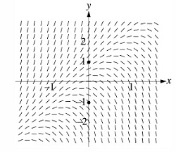
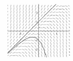
But the question did not stop there, as we shall see, using the slope field could help in other parts of the question.

Part c: Taking these out of order, we will return to part b in a moment. Part c told students that there was a number b for which y = 2x + b is a solution to the differential equation. Students were required to find the value of b and (of course) justify their answer.

There are two approaches. Since y = 2x + b is a solution, we can substitute it into the differential equation and solve for b. Since for this solution dy/dx = 2 we have

$2=2\left( 2x+b \right)-4x$

$2=4x+2b-4x$

$1=b$

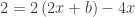
So b = 1 and the solution serves as the justification.

The other method, I’m happy to report, had some students using the slope field. They noticed that the solution through the point (0, 1) is, or certainly appears to be, the line y = 2x + 1. So students guessed that b = 1 and then checked their guess by substituting y = 2x + 1 into the differential equation:

$2=2\left( 2x+1 \right)-4x$

$2=4x+2=4x$

$2=2$

The solution checks and the check serves as the justification.

I like the second solution much better, because it uses the slope field as slope field are intended to be used.

Incidentally, this part was included because readers noticed in previous years that many students did not understand that the solution to a differential equation could be substituted into the differential equation to obtain a true equation as was necessary using either method for part b.

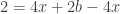
There is yet another approach. Since the solution is given as linear the second derivative must by 0. So

$\displaystyle \frac{{{d}^{2}}y}{d{{x}^{2}}}=2\frac{dy}{dx}-4=2\left( 2y-4x \right)-4$

$2\left( 2y-4x \right)-4=0$

$4y-8x-4=0$

$4y=8x+4$

$y=2x+1$

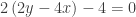
And again b = 1

Returning to part b.

Part b asked students to do an Euler’s method approximation of f(0.2) with two equal steps of the solution of the differential equation through (0, 1). The computation looks like this:

$f\left( 0.1 \right)\approx 1+\left( 2\left( 1 \right)-4\left( 0 \right) \right)\left( 0.1 \right)=1.2$

$f\left( 0.2 \right)\approx 1.2+\left( 2\left( 1.2 \right)-4\left( 0.1 \right) \right)\left( 0.1 \right)=1.4$

So far so good. But this is is about the solution through the point (0, 1). Again referring to the slope field, there is no reason to approximate (except that students were specifically told to do so). Substituting into y = 2x + 1, f(0.2) = 1.4 exactly!

Part d: In the last part of the question students were asked to consider a solution of the differential, g, that satisfied the initial condition g(0) = 0, a solution containing the origin. Students were asked to determine if g(x) had a local extreme at the origin and, if so, to tell what kind (maximum or minimum), and to justify their answer.

Looking again at the slope field it certainly appears that there is a maximum at the origin, and since substituting (0, 0) into the differential equation gives dy/dx = 2(0) – 4(0) = 0, it appears there could be an extreme there. So now how do we determine and justify if this is a maximum or minimum? We cannot use the Candidates’ Test (Closed Interval Test) since we do not have a closed interval, nor can we easily determine if there are any other points nearby where the derivative is zero (there are). Therefore, the First Derivative Test does not help. That leaves the Second Derivative Test.

To use the Second Derivative Test we must use implicit differentiation. (Notice that two unexpected topics now appear extending the scope of the question in a new direction).

$\displaystyle \frac{{{d}^{2}}y}{d{{x}^{2}}}=2\frac{dy}{dx}-4$

At the origin dy/dx = 0 as we already determined, so

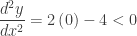
$\displaystyle \frac{{{d}^{2}}y}{d{{x}^{2}}}=2\left( 0 \right)-4<0$

Therefore, since at x = 0, the first derivative is zero and the second derivative is negative the function g(x) has a maximum value at (0, 0) by the Second Derivative Test .

More: Can we solve the differential equation? Yes. The solution has two parts. First we solve the homogeneous differential equation $\frac{dy}{dx}=2y$ , ignoring the –4x for the moment. This is easily solved by separating the variables $y=C{{e}^{2x}}$ , which can be checked by substituting.

Because the differential equation contains x and y and ask ourselves what kind of function might produce a derivative of 2y – 4x? Then we assume there is a solution of the form y = Ax + B where A and B are to be determined and proceed as follows.

$\displaystyle \frac{dy}{dx}=2y-4x$

$A=2\left( Ax+B \right)-4x=\left( 2A-4 \right)x+2B$

Equating the coefficients of the like terms we get the system of equations:

$A=2B$

$0=2A-4$

$A=2\text{ and }B=1$

Putting the two parts together the solution is $y=C{{e}^{2x}}+2x+1$ . This may be checked by substituting. Notice that when C = 0 the particular solution is y = 2x + 1, the line through the point (0, 1).

(Extra: It is not unreasonable to think that instead of y = Ax + B we should assume that the solution might be of the form y = Ax² + Bx + C. Substitute this into the differential equation and show why this is not the case; i.e. show that A = 0, B = 2 and C = 1 giving the same solution as just found.)

Using a graphing program like Winplot, we can consider all the solutions. Below the slope field is graphed using a slider for C to animate the different solutions. The video below shows this with the animation pausing briefly at the two solutions from part a. Notice the maximum point as the graphs pass through the origin.

But wait! There’s more!

The next post will take this question further – Look for it soon.

Update June 27, 2015. Third solution to part c added.

Good Question 1: 2008 AB 6

Posted on January 21, 2015 by Lin McMullin

When I started this blog several years ago I was hoping my readers would ask questions that we could discuss or submit ideas for additional topics to write about. This has not really happened, but I’m still very open to the idea. (That was a HINT.) Since that first year when I had the entire curriculum ahead of me, I have written less not because I dislike writing, but because I am low on ideas.

The other day, I answered a question posted on the AP Calculus Community bulletin board about AB calculus exam question. It occurred to me that this somewhat innocuous looking question was quite good. So I decided to start an occasional series on good questions, from AP exams or elsewhere, that can be used to teaching beyond the actual things asked in the question. (My last post might be in this category, but that was written several months ago.)

In discussing these questions, I will make numerous comments about the question and how to take it further in your class. My idea is not just to show how to write a good answer, but rather to use the question to look deeper into the concepts involved.

Good Question #1: 2008 AB Calculus exam question 6.

The stem gave students the function $\displaystyle f\left( x \right)=\frac{\ln \left( x \right)}{x},\quad x>0$ . Students were also told that $\displaystyle {f}'\left( x \right)=\frac{1-\ln \left( x \right)}{{{x}^{2}}}$ .

The first thought that occurs is why they gave the derivative. The reason is, as we will see, that the first derivative is necessary to answer the first three parts of the question. Therefore, a student who calculates an incorrect derivative is going to be in big trouble (and the readers may have a great deal of work to do reading with the student’s incorrect work). The derivative is calculated using the quotient rule, and students will have to demonstrate their knowledge of the quotient rule later in this question; there is no reason to ask them to do the same thing twice.
If you are using this with a class, you can, and probably should, ask your students to calculate the first derivative. Then you can see how many giving the derivative would have helped.
When discussing the stem, you should also discuss the domain, x > 0, and the x-intercept (1, 0). Other features of the graph, such as end behavior, are developed later in the question, so they may be put on hold briefly.

Part a asked students to write an equation of the tangent line at x = e². To do this students need to do two calculations: $\displaystyle f\left( {{e}^{2}} \right)=\frac{2}{{{e}^{2}}}$ and $\displaystyle {f}'\left( {{e}^{2}} \right)=-\frac{1}{{{e}^{4}}}$ . An equation of the tangent line is $\displaystyle y=\frac{2}{{{e}^{2}}}-\frac{1}{{{e}^{4}}}\left( x-{{e}^{2}} \right)$ .

Writing the equation of a tangent line is a very important skill and should be straightforward. The point-slope form is the way to go. Avoid slope-intercept.
The tangent line is used to approximate the value of the function near the point of tangency; you can throw in an approximation computation here.
After doing part c, you should return here and discuss whether the approximation is an overestimate or an underestimate and how you can tell. (Answer: underestimate, since the graph is concave up here.)
After doing part c, you can also ask them to write the tangent line at the point of inflection and whether approximations near the point of inflection are overestimates or an underestimates, and why. (Answer: Since the concavity change here, it depends on which side of the point of inflection the approximation is made. To the left is an overestimate; to the right is an underestimate.)

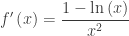Part b asked students to find the x-coordinate of the critical point, determine whether it is a maximum, a minimum, or neither, and to “justify your answer.” To earn credit students had to write the equation $\displaystyle {f}'\left( x \right)=0$ and solve it getting x = e. They had to state that this is a maximum because “ ${f}'\left( x \right)$ changes from positive to negative at x = e.”

This is a very standard AP exam question. To expand it in your class:

Discuss how you know the derivative changes sign here. This will get you into the properties of the natural logarithm function.
Discuss why the change in sign tells you this is a maximum. (A positive derivative indicates an increasing function, etc.)
After doing part c, you can return here and try the second derivative test.
The question asks for “the” critical point, hinting that there is only one. Students should learn to pick up on hints like this and be careful if their computation produces more or less than one.
At this point we have also determined that the function is increasing on the interval $\left( -\infty ,e \right]$ and decreasing everywhere else. The question does not ever ask this, but in class this is worth discussing as important features of the graph. On why these are half-open intervals look here.

Part c told students there was exactly one point of inflection and asked them to find its x-coordinate. To do this they had to use the quotient rule to find that $\displaystyle {{f}'}'\left( x \right)=\frac{-3+2\ln \left( x \right)}{{{x}^{3}}}$ , set this equal to zero and find the x-coordinate to be x = e^3/2.

The question did not require any justification for this answer. In class you should discuss what a justification would look like. The reason is that the second derivative changes sign here. So now you need to discuss how you know this.
Also, you can now determine that the function is concave down on the interval $\left( -\infty ,{{e}^{3/2}} \right)$ and concave up on the interval $\left({{e}^{3/2}},\infty \right)$ . Ask your class to justify this.

Part d asked student to find $\displaystyle \underset{x\to 0+}{\mathop{\lim }}\,\frac{\ln \left( x \right)}{x}$ . The answer is $-\infty$ . While this seems almost like a throwaway tacked on the end because they needed another point, it is the reason I like this question.

The question is easily solved: $\displaystyle \underset{x\to 0+}{\mathop{\lim }}\,\frac{\ln \left( x \right)}{x}=\underset{x\to 0+}{\mathop{\lim }}\,\frac{1}{x}\cdot \underset{x\to 0+}{\mathop{\lim }}\,\ln \left( x \right)=\left( \infty \right)\left( -\infty \right)=-\infty$ .
While tempting, the limit cannot be found by L’Hôpital’s Rule, because on substitution you get $\frac{-\infty }{0}$ ,which is not one of the forms that L’Hôpital’s Rule can handle.
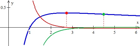
The reason I like this part so much is that we have already developed enough information in the course of doing the problem to find this limit! The function is increasing and concave down on the interval $\left( -\infty ,e \right)$ . Moving from the maximum to the left, the function crosses the x-axis at (1, 0), keeps heading south, and gets steeper. So the limit as you approach the y-axis from the right is negative infinity.This is the left-side end behavior.
What about the right-side end behavior? (You ask your class.) Well, the function is positive and decreasing to the right of the maximum and becomes concave up after x = e^3/2. Thus, it must flatten out and approach the x-axis as an asymptote.
That $\displaystyle \underset{x\to \infty }{\mathop{\lim }}\,\frac{\ln \left( x \right)}{x}=0$ is clear from the note immediately above. This limit can be found by L’Hôpital’s Rule since it is an indeterminate of the type $\infty /\infty$ . So, $\displaystyle \underset{x\to \infty }{\mathop{\lim }}\,\frac{\ln \left( x \right)}{x}=\underset{x\to \infty }{\mathop{\lim }}\,\frac{\tfrac{1}{x}}{1}=0$ .
Notice also that the first derivative approaches zero as x approaches infinity. This indicates that the function’s graph approaches the horizontal as you travel farther to the right. The second derivative also approaches zero as x approaches infinity indicating that the function’s graph is becoming flatter (less concave).

This question and the discussion is largely done analytically (working with equations). We did find a few important numbers in the course of the work. Hopefully, you students discussed this with many good words. To complete the Rule of Four, here is the graph.

And here is a close up showing the important features of the graph and the corresponding points on the derivatives.

The function is shown in blue, the derivative and maximum in red, and the second derivative and the point of inflection in green.

Finally, this function and the limit at infinity is similar to the more pathological example discussed in the post of October 31, 2012 entitled Far Out!

The Marble and the Vase

Posted on October 23, 2014 by Lin McMullin

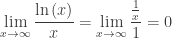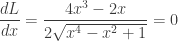
A fairly common max/min problem asks the student to find the point on the parabola $f\left( x \right)={{x}^{2}}$ that is closest to the point $A\left( 0,1 \right)$ . The solution is not too difficult. The distance, L(x), between A and the point $\left( x,{{x}^{2}} \right)$ on the parabola is given by

$\displaystyle L\left( x \right)=\sqrt{{{\left( x-0 \right)}^{2}}+{{\left( {{x}^{2}}-1 \right)}^{2}}}=\sqrt{{{x}^{4}}-{{x}^{2}}+1}$

And the minimum distance can be found when

$\displaystyle \frac{dL}{dx}=\frac{4{{x}^{3}}-2x}{2\sqrt{{{x}^{4}}-{{x}^{2}}+1}}=0$

This occurs when $x=0,\frac{1}{\sqrt{2}},-\frac{1}{\sqrt{2}}$ . The local maximum is occurs when x = 0. The (global) minimums are the other two values located symmetrically to the y-axis.

_________________________

Somewhere I saw this problem posed in terms of a marble dropped into a vase shaped like a parabola. So I think of it that way. This accounts for the title of the post. The problem is, however, basically a two-dimensional situation.

In this post I would like to expand and explore this problem. The exploration will, I hope, give students some insight and experience with extreme values, and the relationship between a graph and its derivative. I will pose a series of questions that you could give to your students to explore. I will answer the questions as I go, but you, of course, should not do that until your students have had some time to work on the questions.

Graphing technology and later Computer Algebra Systems (CAS) will come in handy.

_________________________

1. Consider a general point $A\left( 0,a \right)$ on the y-axis. Find the x-coordinates of the closest point on the parabola in terms of a.

The distance is now given by

$\displaystyle L\left( x \right)=\sqrt{{{\left( x-0 \right)}^{2}}+{{\left( {{x}^{2}}-a \right)}^{2}}}=\sqrt{{{x}^{4}}+\left( 1-2a \right){{x}^{2}}+{{a}^{2}}}$

$\displaystyle \frac{dL}{dx}=\frac{2{{x}^{3}}+\left( 1-2a \right)x}{\sqrt{{{x}^{4}}+2\left( 1-2a \right){{x}^{2}}+{{a}^{2}}}}$

And $\frac{dL}{dx}=0$ when $x=0,\frac{\sqrt{2\left( 2a-1 \right)}}{2},-\frac{\sqrt{2\left( 2a-1 \right)}}{2}$

The (local) maximum is at x = 0. The other values are the minimums. The CAS computation is shown at the end of the post. This is easy enough to do by hand.

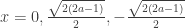
2. Discuss the equation ${{L}^{2}}={{x}^{2}}+{{\left( x-a \right)}^{2}}$ in relation to this situation.

This is the equation of a circle with center at A with radius of L. At the minimum distance this circle will be tangent to the parabola.

3. What happens when $a=\tfrac{1}{2}$ and when $a<\tfrac{1}{2}$ ?

When $a=\tfrac{1}{2}$ , the three zeroes are the same. The circle is tangent to the parabola at the origin and a is the minimum distance.

When $a<\tfrac{1}{2}$ , the circle does not intersect the parabola. Notice that in this case two of the roots of $\frac{dL}{dt}=0$ are not Real numbers.

4. Consider the distance, L(x), from point A to the parabola. As x moves from left to right describe how this length changes. Be specific. Sketch the graph of this distance y = L(x). Where are its (local) maximum and minimum values, relative to the parabola and the circle tangent to the parabola?

The clip below illustrates the situation. The two segments marked L(x) are congruent. The graph of y = L(x) is a“w” shape similar to but not quartic polynomial. The minimums occur directly under the points of tangency of the circle and the parabola. The local maximum is directly over the origin. Is it coincidence that the graph goes through the center of the circle? Explain.

5. Graph $y=\frac{dL}{dx}$ and compare its graph with the graph of $y=L(x)$

L(x) is the blue graph and and L'(x) is the orange graph.
Notice the concavity of L'(x)

6. The graph of $y=\frac{dL}{dx}$ appears be concave up, then down, then (after passing the origin) up, and then down again. There are three points of inflection. Find their x-coordinates in terms of a. How do these points relate to y = L(x) ? (Use a CAS to do the computation)

The points of inflection of the derivative can be found from the second derivative of the derivative (the third derivative of the L(x)). The abscissas are $x=-\sqrt{a},x=0,\text{ and }\sqrt{a}$ . The CAS computation is shown below

CAS Computation for questions 1 and 6.

More Gold

Posted on July 17, 2013 by Lin McMullin

Last week I discussed Lin McMullin’s Theorem (that would be me). The theorem finds where the Golden Ratio shows up in any fourth-degree polynomial. Shortly after that began making the rounds, I got an e-mail from David Tschappat who was then a senior in college. He is now a doctoral student working for an online learning solutions provider.

He related the discovery of a similar appearance of the Golden Ratio in cubic polynomials! Here is his theorem and two other related facts about cubic polynomials (lemmas really) as developed by me.

All cubic polynomials are symmetric to their point of inflection. Therefore, we can simplify matters by translating any cubic so that its point of inflection is at the origin. The general equation will then be $f\left( x \right)=k{{x}^{3}}-3{{h}^{2}}kx$ .

I choose this rather unusual form so that the x-coordinates of the extreme points will be “nice” variables, namely h and –h the zeros of ${f}'\left( x \right)=3k{{x}^{2}}-3{{h}^{2}}k=3k\left( x-h)(x+h \right)$ . The leading coefficient k will eventually divide out and not be a concern.

Now consider two other values x = –2h and x = 2h. So, assuming h > 0, there are five evenly spaced values $-2h<-h<0<h<2h$ that we will consider.

The first two results I will leave as an exercise, as they say:

$f\left( -2h \right)=f\left( h \right)$ and $f\left( -h \right)=f\left( 2h \right)$ . This means that the extreme values are the same as a point on the graph 3h units away on the other side of the y-axis. This is mildly interesting in itself. The reason it is mentioned id that we will use these points soon.
${f}'\left( -2h \right)={f}'\left( 2h \right)$ which is really true for any points at equal distances on opposite sides of the origin. This is obvious from the symmetry of the cubic.

Now comes the interesting and strange part. An equation of a line through one extreme point with a slope equal to that at the point with the same y-coordinate on the other side of the origin (or for that matter the point h units farther away on the same side of the y-axis) is

$y=f\left( -h \right)+{f}'\left( 2h \right)\left( x-\left( -h \right) \right)$

$y=\left( k{{\left( -h \right)}^{3}}-3{{h}^{2}}k\left( -h \right) \right)+\left( 3k{{\left( 2h \right)}^{2}}-3{{h}^{2}}k \right)\left( x+h \right)$

$y=k\left( 11{{h}^{3}}+9{{h}^{2}}x \right)$

Now find where this line intersect the original cubic by solving $y=f\left( x \right)$ . The equation can be solved by hand. We know that x = h is one solution. Synthetic division will give a quadratic and the quadratic formula will do the rest.

$k\left( 11{{h}^{3}}+9{{h}^{2}}x \right)=k{{x}^{3}}-3{{h}^{2}}kx$

$0={{x}^{3}}-12{{h}^{2}}x-11{{h}^{3}}$

$0=\left( x-h \right)\left( {{x}^{2}}+hx-11{{h}^{2}} \right)$

$\displaystyle x=h,\frac{1+3\sqrt{5}}{2}h,\frac{1-3\sqrt{5}}{2}h$

What? You were expecting the Golden Ratio? Not to worry; it’s there!

$\displaystyle \Phi \left( -h \right)+\phi \left( 2h \right)=\frac{1+\sqrt{5}}{2}\left( -h \right)+\frac{1-\sqrt{5}}{2}\left( 2h \right)=\frac{1-3\sqrt{5}}{2}h$

$\displaystyle \Phi \left( 2h \right)+\phi \left( -h \right)=\frac{1+\sqrt{5}}{2}\left( 2h \right)+\frac{1-\sqrt{5}}{2}\left( -h \right)=\frac{1+3\sqrt{5}}{2}h$

Where $\displaystyle \Phi =\frac{1+\sqrt{5}}{2}$ is the Golden Ratio and $\displaystyle \phi ={{\Phi }^{-1}}=\frac{1-\sqrt{5}}{2}$ is the reciprocal of the Golden Ratio.

A similar computation using the other extreme point gives similar results.

Yes, the Golden Ratio is there; I don’t know why it should be there, but it is.

Thank you, David.

Variations on a Theme by ETS

Posted on June 14, 2013 by Lin McMullin

Experienced AP calculus teacher use as many released exam questions during the year as they can. They are good questions and using them gets the students used to the AP style and format. They can be used “as is”, but many are so rich that they can be tweaked to test other concepts and to make the students think wider and deeper.

Below is a multiple-choice question from the 2008 AB calculus exam, question 9.

The graph of the piecewise linear function f is shown in the figure above. If $\displaystyle g\left( x \right)=\int_{-2}^{x}{f\left( t \right)\,dt}$ , which of the following values is the greatest?

(A) g(-3) (B) g(-2) (C) g(0) (D) g(1) (E) g(2)

I am now going to suggest some ways to tweak this question to bring out other ideas. Here are my suggestions. Some could be multiple-choice others simple short constructed response questions. A few of these questions, such as 3 and 4, ask the same thing in different ways.

1. 1. Require students to show work or justify their answer even on multiple-choice questions. So for this question they should write, “The answer is (D) g(1) since x = 1 is the only place where ${g}'\left( x \right)=f\left( x \right)$ changes from positive to negative.”
  2. Ask, “Which of the following values is the least?” (Same choices)
  3. Find the five values listed.
  4. Put the five values in order from smallest to largest.
  5. If $\displaystyle g\left( x \right)=g\left( -2 \right)+\int_{-2}^{x}{f\left( t \right)dt}$ and the maximum value of g is 7, what is the minimum value?
  6. If $\displaystyle g\left( x \right)=g\left( -2 \right)+\int_{-2}^{x}{f\left( t \right)dt}$ and the minimum value of g is 7, what is the maximum value?
  7. Pick any number (not just an integers) in the interval [–3, 2] to be a and change the stem to read, “If $\displaystyle g\left( x \right)=g\left( a \right)+\int_{a}^{x}{f\left( t \right)dt}$ ….” And then ask any of the questions above – some answers will be different, some will be the same. Discussing which will not change and why makes a worthwhile discussion.
  8. Change the equation in the stem to $\displaystyle g\left( x \right)=3x+\int_{-2}^{x}{f\left( t \right)dt}$ and ask the questions above. Again most of the answers will change. Also this question and the next start looking like some free-response questions. Compare them with 2011 AB 4 and 2010 AB 5(c)
  9. Change the equation in the stem to $\displaystyle g\left( x \right)=-\tfrac{3}{2}x+\int_{-2}^{x}{f\left( t \right)dt}$ and ask the questions above. This time most of the answers will change.
  10. Change the graph and ask the same questions.

Not all questions offer as many variations as this one. For some about all you can do is use them “as is” or just change the numbers.

Any other adaptations you can think of?

What is your favorite question for tweaking?

Math in the News Combinatorics and UPS

Revised: August 24, 2014

A Standard Problem?

Posted on May 14, 2013 by Lin McMullin

Sometimes even the simplest problems can lead to interesting places. I got interested in this ordinary textbook problem a few months ago while observing an AB calculus class. Here is how my thinking went written as a series of exercises:

Original exercise: Find the point(s) on the parabola y = x² that are closest to the point (0, 2).

The solution is straightforward:

Let z(x) be the distance from (0, 2) to the point (x, x²). Then $\displaystyle z\left( x \right)=\sqrt{{{\left( x-0 \right)}^{2}}+{{\left( {{x}^{2}}-2 \right)}^{2}}}$ and setting the derivative equal to zero, we find the critical points at x = 0 a local maximum and $x=-\sqrt{\tfrac{3}{2}}$ and $x=\sqrt{\tfrac{3}{2}}$ both absolute minimums located symmetrically to the y-axis.

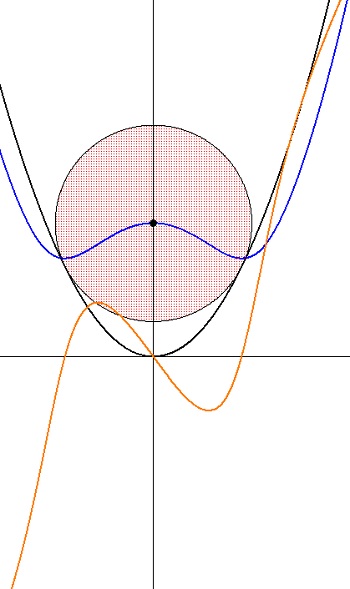
The students had some trouble understanding what was going on. I suggested they consider a point moving along the parabola starting high on the left side. As the point comes down the graph its distance from $\left( 0,2 \right)$ gets shorter until it reaches some minimum length somewhere. Then the distance gets longer again until – where? Obviously, at the origin. Then symmetry takes over and the distance decreases again until it reaches a second minimum directly across the y-axis from the first point, after which it increases forever.

Exercise 1: Sketch the graph of the distance function, z(x), on top of the graph of the parabola. Give the exact coordinates of the maximum point without doing any computations. Discuss the y-coordinates of the minimum points.

It then occurred to me that there is nothing sacred about (0, 2). We could use any point on the y-axis, . Or could we? I pictured a circle centered at the point (0, a) on the y-axis tangent to the parabola (i.e. tangent to the tangent line of the parabola). The radius of such a circle is the minimum distance for that y-axis center point.

Exercise 2: If the point is below the origin then obviously the minimum distance is the distance directly up to the origin. There are places above the x-axis where the origin is the closest point. For what values of a is the origin the closest point? Use the circle mentioned above to explain how this is possible.

The distance graph that we drew above has a W shape similar to the shape of some 4^th degree polynomials (note: z(x) is not a 4^th degree polynomial, it is not even a polynomial). So next I drew the graph of z’(x), the first derivative of z; this graph is similar to a cubic polynomial (again it is not a polynomial)

Exercise 3: Without actually computing the derivative’s equation, sketch the graph of the derivative with the graph of the parabola and the distance function’s graph. Be sure the critical points are where they should be.

Exercise 4: Use a graphing program or a graphing calculator do draw the parabola, z(x) and z’(x) and use it to check your sketches.

Project: Using a suitable program (Winplot, Geogebra, etc.) set up an animation that will show all the features discussed above. It should show the parabola which does not move, the movable point (0, a), the circle tangent to the parabola, z(x) and z’(x). These last 3 should move with the slider for a.

At this point I noticed that the derivative changed concavity 4 times (up-down-up-down). The origin is one of 3 points of inflection. I wondered if there was anything interesting about the location of the points of inflection.

Exercise 5: Find the coordinates of the points of inflection of z’(x). Are they related to any of the features in the problem? (Use a CAS for this one.)

The solutions can be found here: Closest Point Problem Solution.

Far Out!

Posted on October 31, 2012 by Lin McMullin

A monster problem for Halloween.

A while ago I suggested you look at $\displaystyle \underset{x\to \infty }{\mathop{\lim }}\,\frac{\ln \left( {{x}^{5}} \right)}{{{x}^{0.02}}}$ , which using the dominance idea is zero. Of course your students may try graphing or a table. Here’s the graph done by a TI-Nspire CAS. Note the scales.

This is not the way to go. Since the function is increasing near the origin, but the limit at infinity is zero there must be a maximum point where the function starts decreasing. And as the expression can never be negative once x > 1, there must be a point of inflection where the graph becomes concave up and can thereafter approach the x-axis from above as a horizontal asymptote. The maximum can be found by hand which makes for some great algebra manipulation practice:

$\displaystyle \frac{d}{dx}\left( \frac{\ln \left( {{x}^{5}} \right)}{{{x}^{0.02}}} \right)=\frac{{{x}^{0.02}}\tfrac{5{{x}^{4}}}{{{x}^{5}}}-\ln \left( {{x}^{5}} \right)\left( 0.02{{x}^{-0.98}} \right)}{{{x}^{0.04}}}$

$\displaystyle \frac{d}{dx}\left( \frac{\ln \left( {{x}^{5}} \right)}{{{x}^{0.02}}} \right)=\frac{{{x}^{-0.98}}\left( 5-\left( 0.10 \right)\ln \left( x \right) \right)}{{{x}^{0.04}}}=\frac{50-\ln \left( x \right)}{10{{x}^{1.02}}}$

Setting this equal to zero and solving gives $x={{e}^{50}}\approx 5.185\times {{10}^{21}}$

The second derivative is $\displaystyle \frac{{{d}^{2}}}{d{{x}^{2}}}\left( \frac{\ln \left( {{x}^{5}} \right)}{{{x}^{0.02}}} \right)=\frac{-510+10.2\ln \left( x \right)}{100{{x}^{2.02}}}$

and is zero when x = $\displaystyle {{e}^{\frac{520}{10.2}}}\approx 1.382\times {{10}^{22}}$

Okay, I skipped a few steps here, but you can challenge your students with that. Since we’re really interested in the solution here more than the solving ,this is really a good place to use a CAS calculator.

The first line in the figure above defines the function to save typing it each time. The second line finds the x-coordinate of the maximum point (how do we know this is a maximum?) and the third finds the x-coordinate of the point of inflection. Much simpler this way!

Take a minute to consider the numbers. They are BIG! In fact, if the units on our graph paper are centimeters, then the maximum point is a little over 5,480 light-years away from the origin! The point of inflection is about 2.665 times farther at more than 14,607 light-years away!

Meanwhile the maximum value is only 91.9699 cm. That’s right centimeters, less than a meter. And the y-coordinate of the point of inflection is about 91.9524 cm. A drop of 0.0175 cm. in a horizontal distance of a little over 9,127 light-years.

Some problems are a lot less scary if done with technology.

Teaching Calculus

The pleasure lies not in discovering the truth, but in searching for it.

Tag Archives: Extreme Value

Good Question 2: 2002 BC 5

Good Question 1: 2008 AB 6

The Marble and the Vase

More Gold

Variations on a Theme by ETS

A Standard Problem?

Far Out!

Share this:

Share this:

Share this:

Share this:

Share this:

Share this:

Share this: