Comparing the Graph of a Function and its Derivative

Posted on September 6, 2016 by Lin McMullin

The fourth in the Graphing Calculator / Technology series

Comparing the graph of a function and its derivative is instructive and necessary in beginning calculus. Today I will show you how you can do this first with Desmos a free online graphing program and then on a graphing calculator. Desmos does this a lot better than graphing calculators, because of the easy use of sliders. CAS calculators also have sliders but they are not as easy to use as Desmos.

Let’s get started. Instead of presenting you with a completed Desmos graph, I will show you how to make you own. One of the things I have found over the years is that it takes some mathematical knowledge to make good demonstration graph and that in itself if useful and instructive. Hopefully, you and your students will soon be able to make your own to show exactly what you want.

Open Desmos and sign into your account; if you don’t have one then register – its free and you can keep your results and even share them with others.

In the first entry line on the left, enter the equation of the function whose graph you want to explore. Call it f(x); that is enter f(x) = your function. Later you will be able to change this to other functions and investigate them, without changing anything else.

On the second line enter the symmetric difference quotient as

$\displaystyle s\left( x \right)=\frac{f\left( x+0.001 \right)-f\left( x-0.001 \right)}{2\left( 0.001 \right)}$

Instead of a variable h, as we did in our last post in this series, enter 0.001. This will graph the derivative without having to calculate the derivative. Of course, you could enter the derivative here if your class has learned how to calculate derivatives. If so, you will have to change this line each time you change the function.

In order to closely compare the function and its derivative, on the next line enter the equation of a vertical segment from a point on the function (a, f(a)) to a point on the derivative (a, s(a)). Desmos does not have a segment operation, but here is how you graph a segment. In general, a segment from (a, b) to (c, d) is entered as the parametric/vector function

$\left( a\cdot t+c\cdot \left( 1-t \right),b\cdot t+d\cdot \left( 1-t \right) \right),\ 0\le t\le 1$

The a, b, c, and d may be numbers or functions. Since our segment is vertical the first coordinate will have a = c and will reduce to a. Here’s what to enter on the third line:

$\left( a,f\left( a \right)\cdot t+s\left( a \right)\cdot \left( 1-t \right) \right)$

(Notice that there is no x in this expression; t is the variable. Also, the f(a) and s(a) may be interchanged.)

When you push enter, you will be prompted to add a slider for a: click to add the slider. A line will appear under the expression which will allow you to set the domain for t: click the endpoints and enter 0 on the left and 1 on the right, if necessary.

That’s it. You’re done. Use the slider to move around the graphs.

Using the graphs

Discuss with your class, or better yet divide them into groups and let them discuss, what they see. Since at this point they are probably new to this provide some hints such as “What happens on the graph of f when s is 0?” or “What is true on s when f is increasing?” or “What happens to the function at the extreme values of the derivative?” Prompt the students to look for increasing and decreasing, concavity, points of inflection, and extreme values. All the usual stuff. Work from the function to the derivative and from the derivative to the function.

Have your students formulate their results as (tentative) theorems. You actually want them to make some mistakes here, so you can help them improve their thinking and wording. For example, one result might be: If the function is increasing, then the derivative is positive. By changing the first function to an example like f(x) = x³ or f(x) = x + sin (x). Help them see that non-negative might be a better choice.

You might try giving different groups different functions and let them compare and contrast their results.

This is very much in line with MPACs 1, 2, 4, and 6.

You can do the same kind of thing with graphing calculators. That is, you can graph the function and its derivative or a difference quotient. The difference is that graphing calculators do not have sliders.

Extra feature: Desmos will graph a point if you enter the coordinates just like you write them: (a, b). The coordinates may be numbers or functions or a combination of both. Try adding two points to your graph one at each the end of the segment between the graphs that will move with the same slider.

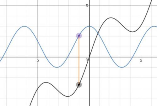
f(x) = x + 2sin(x) and its derivative.

Seeing Difference Quotients

Posted on August 30, 2016 by Lin McMullin

Third in the graphing calculator series.

In working up to the definition of the derivative you probably mention difference quotients. They are

The forward difference quotient (FDQ): $\displaystyle \frac{f\left( x+h \right)-f\left( x \right)}{h}$

The backwards difference quotient (BDQ): $\displaystyle \frac{f\left( x \right)-f\left( x-h \right)}{h}$ , and

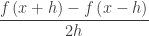
The symmetric difference quotient (SDQ): $\displaystyle \frac{f\left( x+h \right)-f\left( x-h \right)}{2h}$

Each of these is the slope of a (different) secant line and the limit of each as, if it exists, is the same and is the derivative of the function f at the point (x, f(x)). (We will assume h > 0 although this is not really necessary; if h < 0 the FDQ becomes the BDQ and vice versa.)

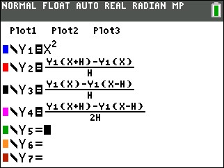
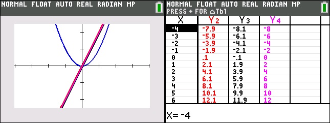
To see how this works you can graph a function and the three difference quotients on a graphing calculator. Here is how. Enter the function as the first function on your calculator and the difference quotients with it. Each of the difference quotients is defined in terms of Y1; this allows us to investigate the difference quotients of different functions by changing only Y1.

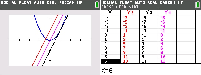
Now, on the home screen assign a value to h by typing [1] [STO] [alpha] [h]

Graph the result in a square window.

The look at the table screen. (Y1 has been turned off). Can you express Y2, Y3, and Y4 in term of x?

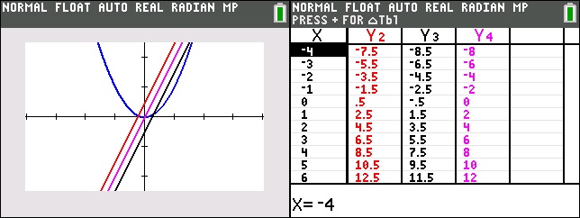
Then change h by storing a different value, say ½, to h and graph again. Then look at the table screen again. Can you express Y2, Y3, and Y4 in term of x?

Then graph again with h = -0.1

As you can see as h gets smaller (h 0), the three difference quotients are FDQ: 2x + h, the BDQ is 2x – h, and the SDQ is 2x. They converge to the same thing. The limit of each difference quotient as h approaches zero is twice the x coordinate of the point. If you’re not sure try a smaller value of h.

The function to which each of these converge is called the derivative of the original function (Y1). In the example the derivative of x² is 2x.

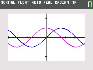
Now try another function say, Y1 = sin(x) and repeat the graphs and tables above. The tables will probably not be of much help, since the pattern is not familiar. The graph shows the function (dark blue) and only the SDQ (light blue), h = 0.1 Can you guess what the derivative might be?

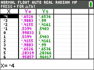
I f you guessed cos(x) you are correct. The table shows the SDQ values as Y4, and the values of cos(x) as Y5. Pretty close! If you want to get closer try h = 0.001.

If you have a CAS calculators such as the TI-Nspire or the HP PRIME you can do this activity with sliders. Also you may try this with DESMOS. Click here or on the graph below. Some interesting functions to start with are cos(x) and | x |.

And by the way, the SDQ is what most graphing calculators use to calculate the derivative. It is called nDeriv on TI calculators.

Tangent Lines

Posted on August 23, 2016 by Lin McMullin

Second in the Graphing Calculator/Technology series

This graphing calculator activity is a way to introduce the idea if the slope of the tangent line as the limit of the slope of a secant line. In it, students will write the equation of a secant line through two very close points. They will then compare their results in several ways.

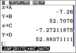
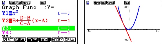
Begin by having the students graph a very simple curve such as y = x² in the standard window of their calculator. Then TRACE to a point. Students will go to different points, some to the left and some to the right of the origin. ZOOM IN several times on this point until their graph appears linear (discuss local linearity here). To be sure they are on the graph push TRACE again. The coordinates of their point will be at the bottom of the screen; call this point (a, b). Return to the home screen and store the values to A and B (click here for instructions on storing and recalling numbers).

Return to the graph and push TRACE again to be sure the cursor is on the graph. Move the TRACE cursor one or two pixels away from the first point in either direction. This new point is (c, d). Return to the home screen and store the coordinates to C and D.

Enter the equation of the line through the two points on the equation entry screen in terms of A, B, C, and D. Zoom Out several times until you have returned to the original window..

Exploration 1: Have students compare and contrast their graphs with several other students and discuss their observations. (Expected observations: the lines appear tangent at each students’ original point)

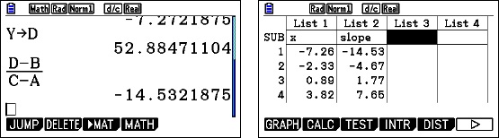
Exploration 2: Ask student to compute the slope of the line through their points, again using A, B, C, and D. Collect each student’s x-coordinate, A, and their slope and enter them in list is your calculator so that they can be projected.

Study the two lists and discuss the relation is any. (Expected observations: the slope is twice the x-coordinate.) Can you write an equation of these pairs? (Expected result: y = 2x)

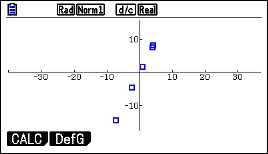
Finally, plot the points on the calculator using a square window. Do the points seem to lie on the line y =2x?

Extensions:

Try the same activity with other functions such as y = (1/3)x³, y = x³, or y = x⁴. Anything more difficult will still result in a tangent line, but the numerical relationship between x and the slope will probably be too difficult to see. You may also consider y = sin(x) or y = cos(x). Again, the numerical work in Exploration 2, will be too difficult to see, but on graphing the points the result may be obvious. For y = sin(x), return to the list and add a column with the cosines of the x-values. Compare these with the slopes.

Graphing Calculator Use

Posted on August 16, 2016 by Lin McMullin

First in a series.

I am going to (try to) write a series of posts this fall on graphing calculator use in for calculus. Graphing calculators became generally available around 1989 and were made a requirement for use on the AP calculus exams in 1995. The hope was that they would encourage the use of technology generally in all math classes, and to an extent this has happened. In the coming posts I hope to show how graphing calculators can be used beyond the four skills required for the AP exams to help students understand what’s going on.

I will occasionally work with CAS calculators, but the main focus will be the basic non-CAS graphing calculators. All the suggestions will work of CAS calculators, of course. Also, I will occasionally make use of Desmos a free online graphing utility that students can easily access on their computer, tablet or smart phone.

Today I will discuss the four things students should be able to do, and in fact are required to do, on the AP exams. I will also show how to store and recall numbers. This last skill, while not required, is very useful. I have found that some teachers, and therefore their students, are unaware of this common feature of graphing calculators.

Calculators and other technology should be available from at least Algebra 1 on. So by the time students get to calculus calculator use (except for the calculus specific operations) should all be second nature to them.

So let’s get going. Here are the four required skills and some brief comments on each.

Graph a function in a suitable window. The exam questions do not say “use a calculator”, so students are expected to know when seeing a graph will help them. The viewing window is not usually specified either so students should be familiar with setting the viewing window. If the domain is given in the question, then that’s what the students should use. If no domain is given, then use a range that includes the answer choices.
Solve an equation numerically. Students may use any built-in feature to do this. The home screen “solver”, a routine called “Poly” or “Poly solve” are all allowed. Probably the most useful is to graph both sides of the equation and then use the graph operation called “intersect” to find the points of intersection one at a time. Another approach is to set the equation equal to 0, graph that expression and use the “roots” or “zeros” operations to solve the equation.
Find the value of the derivative of a function at a given point. There is a built-in template for this.
Find the value of a definite integral. There is a built-in template for this also.

Store-and-Recall

I will demonstrate the store-and-recall idea with an example that will also use skill 1, 2, and 4 from the list above.

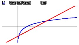
Example: Find the area between the graph of f(x) = ln(x) and g(x) = x – 2, using (1) vertical rectangles, and (2) using horizontal rectangles.

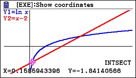
For either method we need the coordinates of the points of intersection of the graphs. So, begin by graphing the functions and adjusting the window so the important points are visible.

Next use the intersection operation to find the first point of intersection.

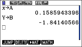
Different calculators will do this slightly differently. The coordinates of the points of intersection are shown at the bottom of the screen. Think of this point as (a, b). The coordinates need to be stored for use later. To do this return to the home screen and type

[x] [STO], [alpha] [A] and [alpha] [y] [STO] [alpha] [B]

If your graph screen shows different names, such as xc and yc, then type that befroe the [STO] key. (The store [STO] key may look like an arrow pointing right.)

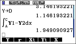
Return to the graph screen and find the coordinates of the second point of intersection; think of this as (c, d). Return to the home screen and store the coordinates as C and D. They are c = 3.146193221 and d = 1.146193221.

To find the area use the definite integral template and enter the information needed. For the vertical rectangles you may use either the function or Y1 and Y2 that you entered to graph.

Notice that the upper and lower limits of integration are A and C. The calculator uses the values you stored in these locations. You can use the variables in any kind of computation.

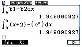
Here is the horizontal rectangle computation using B and D as limits. The functions solved for y are x = y + 2 on the right and x = e^y on the left. (The y’s have been changed to x’s since the template only allows x as a variable.)

Notice that so far, we’ve written nothing down. Everything has been done on the calculator. This prevents copy errors and round-off errors.

What should a student show on his or her AP Exam? They are required to show what they are doing, or more precisely what they’ve asked their calculator to do. They need to write the equation they are solving with the solution next to it, but no intermediate work. They should indicate what A and C are. So

$\ln (x)=x+2,\ x=0.158594\text{ and }x=3.146193$

$a=0.158594\text{ and }c=3.146193$

Then show the integral and answer. Here again they may use f and g given in the stem or the actual expressions. There is no requirement that answers must be given to three decimal places, so there is no need to round.

$\displaystyle \int_{a}^{c}{f\left( x \right)-g\left( x \right)dx}=1.94909$

The next post in this series will show you a way to introduce the idea odf the derivative as the slope of the tangent line.

Back to School – 2016

Posted on August 10, 2016 by Lin McMullin

BACK TO SCHOOL – The three words we love and we hate.

I’ve been touching up the blog a bit this week. I hope the changes will make it easier to find posts on the topics you are interested in, and the blog more useful in general.

The THRU THE YEAR tab on the navigation bar at the top of the page has been updated. Links to my videos are now included. The monthly listings are organized so that you can stay ahead of your syllabus; to give you time to incorporate a new idea you like. So if your school starts in September, the August posts are where to start. The order of topics is not a day-to-day listing for you to follow or not even the order you must teach them in. So feel free to look around and rearrange.

The latest post appears at the top of the page. Below that are the four FEATURED POSTS. I will keep the current group in place for a while. These four posts concern the new Course and Exam Description (CED) for the AP Calculus program. The AP Calculus Concept Outline and the Mathematical Practices will be a help you understand the AP courses. The Getting Organized post will show you a way to organize your course using a Trello board that is already started for you.

Below the Featured Posts are the latest posts, newest on top. At the end of each post is a comment button so you can add your comments, suggestions, and ideas. Please use it.

You can find topics by using the SEARCH box on the right below the featured posts. Below that is a POST BY TOPIC drop-down list and a chronological ARCHIVES drop-down list.

If you cannot find what you need please let me know and I’ll see what I can do to help. I really could use some suggests for posts. My email is lnmcmullin@aol.com.

My plan for the coming months is to write posts on simple graphing calculator use for AP Calculus – ideas that I hope you can use to help your students understand what’s going on better. Look for them.

I hope the blog will make your year a little easier.

Have a good one!

Parts and More Parts

Posted on August 5, 2016 by Lin McMullin

At an APSI this summer the participants and I got to discussing the “tabular method” for integration by parts. Since we were getting far from what is tested on the BC Calculus exams, I ended the discussion and said for those that were interested I would post more on the tabular method this blog going farther than just the basic set up. So here goes.

Here are some previous posts on integration by parts and the tabular method

Integration by Parts 1 discusses the basics of the method. This is as far as a BC course needs to go.

Integration by Parts 2 introduces the tabular method

Modified Tabular Integration presents a very quick and slick way of doing the tabular method without making a table. This is worth knowing.

There is also a video on integration by parts here. Scroll down to “Antiderivatives 5: A BC topic – Integration by parts.” The tabular method is discussed starting about time 15:16. There are several ways of setting up the table; one is shown here and a slightly different way is in the Integration by Parts 2 post above. There are others.

Going further with the tabular method.

The tabular method works well if one of the factors in the original integrand is a polynomial; eventually its derivative will be zero and you are done. These are shown in the examples in the posts above and Example 1 below. To complete the topic, this post will show two other things that can happen when using integration by parts and the tabular method.

First we look at an example with a polynomial factor and learn how to stop midway through. Why stop? Because often there will be no end if you don’t stop. There are ways to complete the integration as shown in the examples.

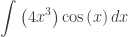
Example 1: Find $\displaystyle \int_{{}}^{{}}{\left( 4{{x}^{3}} \right)\cos \left( x \right)dx}$ by the tabular method (See Integration by Parts 2 for more detail on how to set the table up)

Adding the last column gives the antiderivative:

$\displaystyle \int_{{}}^{{}}{\left( 4{{x}^{3}} \right)\cos \left( x \right)dx}=4{{x}^{3}}\sin \left( x \right)+12{{x}^{2}}\cos \left( x \right)-24x\sin \left( x \right)-24\sin \left( x \right)+C$

Now say you wanted to stop after $12{{x}^{2}}\cos \left( x \right)$ . Example 2 shows why you want (need) to stop. In Example 1 you will have

$\displaystyle \int_{{}}^{{}}{\left( 4{{x}^{3}} \right)\cos \left( x \right)dx}=4{{x}^{3}}\sin \left( x \right)+12{{x}^{2}}\sin \left( x \right)+\int_{{}}^{{}}{-24x\cos \left( x \right)}dx$

The integrand on the right is the product of the last column in the row at which you stopped and the first two columns in the next row, as shown in yellow above.

Example 2 Find $\displaystyle \int_{{}}^{{}}{{{e}^{x}}\cos \left( x \right)dx}$

As you can see things are just repeating the lines above sometimes with minus signs. However, if we stop on the third line we can write:

$\displaystyle \int_{{}}^{{}}{{{e}^{x}}\cos \left( x \right)dx={{e}^{x}}\sin \left( x \right)}+{{e}^{x}}\cos \left( x \right)-\int_{{}}^{{}}{{{e}^{x}}\cos \left( x \right)dx}$

The integral at the end is identical to the original integral. We can continue by adding the integral to both sides:

$\displaystyle 2\int_{{}}^{{}}{{{e}^{x}}\cos \left( x \right)dx={{e}^{x}}\sin \left( x \right)}+{{e}^{x}}\cos \left( x \right)$

Finally, we divide by 2 and have the antiderivative we were trying to find:

$\displaystyle \int_{{}}^{{}}{{{e}^{x}}\cos \left( x \right)dx=\tfrac{1}{2}{{e}^{x}}\sin \left( x \right)}+\tfrac{1}{2}{{e}^{x}}\cos \left( x \right)+C$

In working this type of problem you must be aware of that the original integrand showing up again can happen and what to do if it does. As long as the coefficient is not +1, we can proceed as above. The same thing happens if we do not use the tabular method. (If the coefficient is +1 then the other terms on the right will add to zero and you need to make different choices for u and dv.)

Reduction Formulas.

Another use of integration by parts is to produce formulas for integrals involving powers. An integral whose integrand is of less degree than the original, but of the same form results. The formula is then iterated to continually reduce the degree until the final integral can be integrated easily.

Example 3: Find $\displaystyle \int_{{}}^{{}}{{{x}^{n}}{{e}^{x}}dx}$

Let $u={{x}^{n}},\ du=n{{x}^{n-1}}dx,\ dv={{e}^{x}}dx,\ v={{e}^{x}}$

$\displaystyle \int_{{}}^{{}}{{{x}^{n}}{{e}^{x}}dx}={{x}^{n}}{{e}^{x}}-n\int_{{}}^{{}}{{{x}^{n-1}}{{e}^{x}}dx}$

This is a reduction formula; the second integral is the same as the first, but of lower degree. Here is how it is used. At each step the integrand is the same as the original, but one degree lower. So the formula can be applied again, three more times in this example.

Most textbooks have a short selection of reduction formulas.

Final Thoughts.

Back in the “old days”, BC (before calculators), beginning calculus courses spent a lot of time on the topic of “Techniques of Integration.” This included integration by parts, algebraic techniques, techniques known as trig-substitutions, and others. Mathematicians and engineers had tables of integrals listing over a thousand forms and students were taught how to use the tables and distinguish between similar forms in the tables. (See the photo below from the fourteenth edition of the CRC tables (c) 1965.) Current textbooks often contain such sections still.

Today, none of this is necessary. CAS calculators can find the antiderivatives of almost any integral. Websites such as WolframAlpha are also available to do this work.

I’m not sure why the College Board recently expanded slightly the list of types of antiderivatives tested on the exams. Certainly a few of the basic types should be included in a course, but what students really need to know is how to write the integral appropriate to a problem, and what definite and indefinite integrals mean. This, in my opinion, is far more important than being able to crank out antiderivatives of increasingly complicated expressions: let technology do that – or buy yourself an integral table. Just saying … .

Summertime

Posted on June 1, 2016 by Lin McMullin

Flowers at Ashford Castle, Ireland.

Well school is over in most of the country, even if the folks here in the Northeast do have a few weeks to go . I am not planning to write much over the summer; I’d like to, but am short on ideas. So if you have any questions, suggestions, or just something from Calculusville you’d like to hear about please let me know, and I’ll see what I can do. My email address is lnmcmullin@aol.com

I have a vacation and then one AP summer institute planned. Other than that, I’m going to perfect my loafing techniques

Since many of you will be planning for next school year and the new Course and Exam Description (CED), I’ll leave the four featured posts below so you can find them easily. The College Board has produced a series of short videos on the new CED. Click here to see these Course Overview Modules.

And take some time off for yourself and your family as well.

Happy Summer.

Teaching Calculus

The pleasure lies not in discovering the truth, but in searching for it.