MPAC 5: Building notational fluency
Students can:
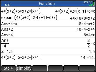
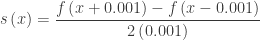
a. know and use a variety of notations (e.g.,
);
b. connect notation to definitions (e.g., relating the notation for the definite integral to that of the limit of a Riemann sum);
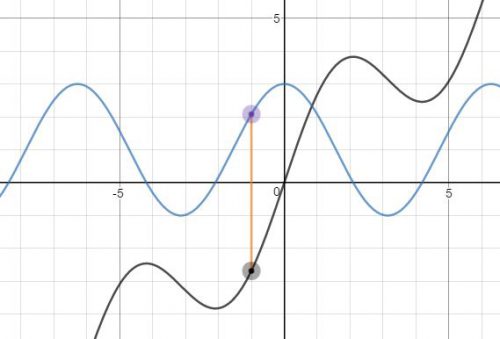
c. connect notation to different representations (graphical, numerical, analytical, and verbal); and
d. assign meaning to notation, accurately interpreting the notation in a given problem and across different contexts.
— AP® Calculus AB and AP® Calculus BC Course and Exam Description Effective Fall 2016, The College Board, New York © 2016. Full text is here.
The use of symbols is, not only what everyone thinks of when they think of mathematics, but quite rightly it’s a great tool. Notation has made the abstraction of diverse mathematical concepts possible and revealed the connections between disparate parts of mathematics. Each notation is defined somewhere; the new notations of the calculus are defined during the course (MPAC 5b). Students often do not realize that notation is simply shorthand. Symbols seem to have a magical quality and do things on their own. It is up to the teacher to demystify all this by making the connections listed in this MPAC for the students and making sure students use the notation properly.
How/where can you make sure students use these ideas in your classes.
The variety of notations and often their redundancy are confusing to students and therefore need to be carefully explained and properly used. This does not begin in calculus, but rather from the first days of students’ mathematical life: the plus sign, +, is notation. Even earlier, 1, 2, 3, are notations. We hope that by the time students get to the calculus they have had a lot of experience with notation and that their teachers have insisted on using notation correctly. The fact that there is often more than one notation for the same thing is recognized in MPAC 5a.
Notation often has meaning related to graphs. For instance, a horizontal asymptote at y = 3 is the graphical manifestation of the expression
Notation speeds up communicating (MPAC 6) about what students are doing. For example, given the velocity expression of a moving object and asked to find the acceleration at t = 5.432, all student need to write is a(5.432) = v’(5.432) = their answer. This not only identifies the answer, but also explains (justifies) what they are doing.
Notation sometimes serves as directions on how to do some process. The Product rule, the Quotient rule and the Chain rule all help us remember what to do when finding derivatives.
But student often misuse notation. A common misuse of notation is to string their computations together with equal signs where that is neither appropriate nor true. They will calculate the integral needed to find the average value over [0,8] and get a decimal answer, say 1034, and then write 1034 = 1034/8 is the average value – correct answer, poor notation, a point lost. Another common mistake is to calculate an area by unwittingly subtracting the upper curve from the lower and get an answer, say –10 and then write –10 = 10. This loses one point for the wrong integrand and another point for the lie –10 = 10. Likewise, saying this integral = |-10| is not correct.
Both examples are incorrect use of the equal sign. Probably the best way to avoid this is to do computation vertically, one line at a time and not connect them with the equal signs. In the first case, had they written
- Correct integral = 1034
- Average value = 1034/8
They earn full credit. In the second example if they write
- Integral lower minus upper = –10 <loses one point>
- Area = 10
- They not only earn the answer point, but regain (recoup in “reader talk”) the point they lost for the wrong integrand, and earn full credit.
The accurate and precise use of notation is also mentioned in MPAC 6.
When AP exam questions are written the writers reference them to the LOs, EKs and MPACs. The released 2016 Practice Exam given out at summer institutes this summer is in the new format and contains very detailed solutions for both the multiple-choice and free-response questions that include these references. (This version is not available online as far as I know.) A little more than 1/3 of the multiple-choice and all six free-response questions on both AB and BC exam reference MPAC 5.
Here are some previous posts on these subjects:
Definition of the Definite Integral

PLEASE NOTE: I have no control over the advertising that appears on this blog. It is provided by WordPress and I would have to pay a great deal to not have advertising. I do not endorse anything advertised here. I noticed that ads for one of the presidential candidates occasionally appears; I certainly do not endorse him.


 in the standard window. The vertical line is not really the asymptote and the “hole” at (2, 0.75) is not seen.