Is this going to be on the exam?

confused-teacherRecently there was a discussion on the AP Calculus Community bulletin board regarding whether it was necessary or desirable to have students do curve sketching starting with the equation and ending with a graph with all the appropriate features – increasing/decreasing, concavity, extreme values etc., etc. – included. As this is kind of question that has not been asked on the AP Calculus exam, should the teacher have his students do problems like these?

The teacher correctly observed that while all the individual features of a graph are tested, students are rarely, if ever, expected to put it all together. He observed that making up such questions is difficult because getting “nice” numbers is difficult.

Replies ran from No, curve sketching should go the way of log and trig tables, to Yes, because it helps connect f. f ‘ and f ‘’, and to skip the messy ones and concentrate on the connections and why things work the way they do. Most people seemed to settle on that last idea; as I did. As for finding questions with “nice” numbers, look in other textbooks and steal borrow their examples.

But there is another consideration with this and other topics. Folks are always asking why such-and-such a topic is not tested on the AP Calculus exam and why not.

The AP Calculus program is not the arbiter of what students need to know about first-year calculus or what you may include in your course. That said, if you’re teaching an AP course you should do your best to have your students learn everything listed in the 2019 Course and Exam Description book and be aware of how those topics are tested – the style and format of the questions. This does not limit you in what else you may think important and want your students to know. You are free to include other topics as time permits.

Other considerations go into choosing items for the exams. A big consideration is writing questions that can be scored fairly.  Here are some thoughts on this by topic.

Curve Sketching

If a question consisted of just an equation and the directions that the student should draw a graph, how do you score it? How accurate does the graph need to be? Exactly what needs to be included?

An even bigger concern is what do you do if a student makes a small mistake, maybe just miscopies the equation? The problem may have become easier (say, an asymptote goes missing in the miscopied equation and if there is a point or two for dealing with asymptotes – what becomes of those points?) Is it fair to the student to lose points for something his small mistake made it unnecessary for him to consider? Or if the mistake makes the question so difficult it cannot be solved by hand, what happens then? Either way, the student knows what to do, yet cannot show that to the reader.

To overcome problems like these, the questions include several parts usually unrelated to each other, so that a mistake in one part does not make it impossible to earn any subsequent points. All the main ideas related to derivatives and graphing are tested somewhere on the exam, if not in the free-response section, then as a multiple-choice question.

(Where the parts are related, a wrong answer from one part, usually just a number, imported into the next part is considered correct for the second part and the reader then can determine if the student knows the concept and procedure for that part.)

Optimization

A big topic in derivative applications is optimization. Questions on optimization typically present a “real life” situation such as something must be built for the lowest cost or using the least material. The last question of this type was in 1982 (1982 AB 6, BC 3 same question). The question is 3.5 lines long and has no parts – just “find the cost of the least expensive tank.”

The problem here is the same as with curve sketching. The first thing the student must do is write the equation to be optimized. If the student does that incorrectly, there is no way to survive, and no way to grade the problem. While it is fair to not to award points for not writing the correct equation, it is not fair to deduct other points that the student could earn had he written the correct equation.

The main tool for optimizing is to find the extreme value of the function; that is tested on every exam. So here is a topic that you certainly may include the full question in you course, but the concepts will be tested in other ways on the exam.

The epsilon-delta definition of limit

I think the reason that this topic is not tested is slightly different. If the function for which you are trying to “prove” the limit is linear, then \displaystyle \delta =\frac{\varepsilon }{\left| m \right|} where m is the slope of the line – there is nothing to do beside memorize the formula. If the function is not linear, then the algebraic gymnastics necessary are too complicated and differ greatly depending on the function. You would be testing whether the student knew the appropriate “trick.”

Furthermore, in a multiple-choice question, the distractor that gives the smallest value of must be correct (even if a larger value is also correct).

Moreover, finding the epsilon-delta relationship is not what’s important about the definition of limit. Understanding how the existence of such a relationship say “gets closer to” or “approaches” in symbols and guarantees that the limit exists is important.

Volumes using the Shell Method

I have no idea why this topic is not included. It was before 1998. The only reason I can think of is that the method is so unlike anything else in calculus (except radial density), that it was eliminated for that reason.

This is a topic that students should know about. Consider showing it too them when you are doing volumes or after the exam. Their college teachers may like them to know it.

Integration by Parts on the AB exam

Integration by Parts is considered a second semester topic. Since AB is considered a one-semester course, Integration by Parts is tested on the BC exam, but not the AB exam. Even on the BC exam it is no longer covered in much depth: two- or more step integrals, the tabular method, and reduction formulas are not tested.

This is a topic that you can include in AB if you have time or after the exam or expand upon in a BC class.

Newton’s Method, Work, and other applications of integrals and derivatives

There are a great number of applications of integrals and derivatives. Some that were included on the exams previously are no longer listed. And that’s the answer right there: in fairness, you must tell students (and teachers) what applications to include and what will be tested. It is not fair to wing in some new application and expect nearly half a million students to be able to handle it.

Also, remember when looking through older exams, especially those from before 1998, that some of the topics are not on the current course description and will not be tested on the exams.

Solution of differential equations by methods other than separation of variables

Differential equations are a huge and important area of calculus. The beginning courses, AB and BC, try to give students a brief introduction to differential equations. The idea, I think, is like a survey course in English Literature or World History: there is no time to dig deeply, but the is an attempt to show the main parts of the subject.


While the choices are somewhat arbitrary, the College Board regularly consults with college and university mathematics departments about what to include and not include. The relatively minor changes in the new course description are evidence of this continuing collaboration. Any changes are usually announced two years in advance. (The recent addition of density problems unannounced, notwithstanding.) So, find a balance for yourself. Cover (or better yet, uncover) the ideas and concepts in the course description and if there if a topic you particularly like or think will help your students’ understanding of the calculus, by all means include it.


PS: Please scroll down and read Verge Cornelius’ great comment below.


Happy Holiday to everyone. There is no post scheduled for next week; I will resume in the new year. As always, I like to hear from you. If you have anything calculus-wise you would like me to write about, please let me know and I’ll see what I can come up with. You may email me at lnmcmullin@aol.com


.

Good Question 12 – Parts with a Constant?

partsSomeone asked me about this a while ago and I thought I would share it with you. It may be a good question to get your students thinking about; see if they can give a definitive answer that will, of course, include a justification.

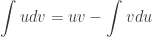
Integration by Parts is summarized in the equation

\displaystyle \int_{{}}^{{}}{udv}=uv-\int_{{}}^{{}}{vdu}

To use the equation, you choose part of a given integral (left side) to be u and part to be dv, both functions of x. Then you differentiate u and integrate dv and use them on the right side to obtain a simpler integral that you can integrate.

The question is this: When you integrate dv, should you, can you, have a constant of integration, the “+ ” that you insist upon in other integration problems? Why don’t you use it here? Or can you?

Scroll down for my answer.

Answer: Let’s see what happens if we use a constant. Assume that \displaystyle \int_{{}}^{{}}{dv}=v+C. Then

\displaystyle \int_{{}}^{{}}{udv}=u\cdot \left( v+C \right)-\int_{{}}^{{}}{\left( v+C \right)du}

\displaystyle =uv+Cu-\left( \int_{{}}^{{}}{vdu}+\int_{{}}^{{}}{Cdu} \right)

\displaystyle =uv+Cu-\int_{{}}^{{}}{vdu}-Cu

\displaystyle =uv-\int_{{}}^{{}}{vdu}

So, you may use a constant if you want, but it will always add out of the expression.


For more on integration by parts see here for the basic idea, here for the tabular method, here for a quicker way than the tabular method, and here for more on the tabular method and reduction formulas.


Subtract the Hole from the Whole.

Sometimes I think textbooks are too rigorous. Behind every Riemann sum is a definite integral. So, authors routinely show how to solve an application of integration problem by developing the method starting from the Riemann sum and proceeding to an integral that give the result that is summarized in a “formula.” There is nothing wrong with that except that often the formula is all the students remember and are lost when faced with a similar situation that the formula does not handle. .

The volume of solid figure problems are developed from the idea that if a solid figure has a regular cross-section (that is, when cut perpendicular to a line, each face is similar – in the technical sense – to all the others). They are all squares, or equilateral triangles, or whatever. The last shape considered is usually a “washer”, that is, an annulus or two concentric circles. This is formed by revolving the region between two curves around a line. Authors develop a formula for such volumes: \displaystyle \pi \int_{a}^{b}{{{\left( R\left( x \right) \right)}^{2}}-{{\left( r\left( x \right) \right)}^{2}}dx}.

Now there is nothing wrong with that, but I like to give the students their chance to show off. They can usually figure out the answer without Riemann sums. Here is my suggestion. After students have had some practice with circular cross-sections (“Disk” method”) I give them a series of three volumes to find.

Example 1: The curve f\left( x \right)=\sin \left( \pi x \right) on the interval [0, ½] is revolved around the x-axis to form a solid figure. Find the volume of this figure. washers-1
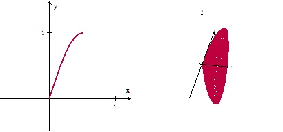
Solution: \displaystyle V=\int_{0}^{1}{\pi {{\left( \sin \left( \pi x \right) \right)}^{2}}dx}=\frac{\pi }{4}

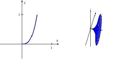
Example 2: The curve g\left( x \right)=8{{x}^{3}} on the interval [0, ½] is revolved around the x-axis to form a solid figure. Find the volume of this figure.   washers-2

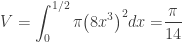
Solution: \displaystyle V=\int_{0}^{1/2}{\pi {{\left( 8{{x}^{3}} \right)}^{2}}dx=}\frac{\pi }{14}

These they find easy. Then, leaving the first two examples in plain view, I give them:

Example 3: The region in the first quadrant between the graphs of f\left( x \right)=\sin \left( \pi x \right) and g\left( x \right)=8{{x}^{3}} is revolved around the x-axis. Find the volume of the resulting figure.washers-3

A little thinking and (rarely) a hint and they have it. \displaystyle V=\frac{\pi }{4}-\frac{\pi }{14}

What did they do? Easy, they subtracted the hole from the whole. We discuss this and why they think it is correct. We try one or two others. And now they are set to do any “washer” method problem without another formula to memorize.


Extensions:

1. In symbols, when rotation around a horizontal line, if R(x) is the distance from the curve farthest from the line of rotation and r(x) the distance from the closer curve to the line of rotation the result can be summarized in the formula

\displaystyle V = \int_{a}^{b}{\pi {{\left( R\left( x \right) \right)}^{2}}dx}-\int_{a}^{b}{\pi {{\left( r\left( x \right) \right)}^{2}}dx}.

         Notice, that I like to keep the \pi  inside the integral sign so that each integrand looks like the formula for the area of a circle. What the students need to know is to subtract the volume hole from the outside volume. With that                idea and the disk method they can do any volume by washers problem.

2. You should show the students how this equation above can be rearranged into the formula in their books,

\displaystyle V = \pi \int_{a}^{b}{{{\left( R\left( x \right) \right)}^{2}}-{{\left( r\left( x \right) \right)}^{2}}dx}.

This is so that they understand that the formulas are the same, and not think you’ve forgotten to tell them something important. It is also a good exercise in working with the notation. (see MPAC 5 – Notational fluency)

3. Next discuss what {{\left( \pi R\left( x \right) \right)}^{2}}-\pi {{\left( r\left( x \right) \right)}^{2}} is the area of and how it relates to this problem. See if the students can understand what the textbook is doing; what shape the book is using.. Discuss the Riemann sum approach. (MPAC 1 Reasoning with definitions and theorems, and MPAC 5 Notational fluency)

4. With the idea of subtracting the “hole” try a problem like this. Example 4: The region in the first quadrant between x-axis and the graphs of f\left( x \right)=\sqrt{x} and g\left( x \right)=\sqrt{2x-4} is revolved around the x-axis. Find the volume of the resulting figure. washers-4

Solution:\displaystyle V=\int_{0}^{4}{\pi {{\left( \sqrt{x} \right)}^{2}}dx}-\int_{2}^{4}{\pi {{\left( \sqrt{2x-4} \right)}^{2}}dx}=4\pi

(Notice the limits of integration.)

Traditionally, this is done by the method of cylindrical shells, but you don’t need that. You could divide the region into two parts with a vertical line at x = 2 and use disks on the left and washers on the right, but you don’t need to do that either. Just subtract the hole from the whole.

.

Good Question 11 – Riemann Reversed

Good Question 11 – or not. double-riemann


The question below appears in the 2016 Course and Exam Description (CED) for AP Calculus (CED, p. 54), and has caused some questions since it is not something included in most textbooks and has not appeared on recent exams. The question gives a Riemann sum and asks for the definite integral that is its limit. Another example appears in the 2016 “Practice Exam” available at your audit website; see question AB 30. This type of question asks the student to relate a definite integral to the limit of its Riemann sum. These are called reversal questions since you must work in reverse of the usual order. Since this type of question appears in both the CED examples and the practice exam, the chances of it appearing on future exams look good.

To the best of my recollection the last time a question of this type appeared on the AP Calculus exams was in 1997, when only about 7% of the students taking the exam got it correct. Considering that by random guessing about 20% should have gotten it correct, this was a difficult question. This question, the “radical 50” question, is at the end of this post.

Example 1

Which of the following integral expressions is equal to \displaystyle \underset{n\to \infty }{\mathop{\lim }}\,\sum\limits_{k=1}^{n}{\left( \sqrt{1+\frac{3k}{n}}\cdot \frac{1}{n} \right)} ?

There were 4 answer choices that we will consider in a minute.

The first key to answering the question is to recognize the limit as a Riemann sum. In general, a right-side Riemann sum for the function f on the interval [a, b] with n equal subdivisions, has the form:

\displaystyle \underset{n\to \infty }{\mathop{\lim }}\,\sum\limits_{k=1}^{n}{\left( f\left( a+\frac{b-a}{n}\cdot k \right)\cdot \frac{b-a}{n} \right)}=\int_{a}^{b}{f\left( x \right)dx}

To evaluate the limit and express it as an integral, we must identify, a, b, and f. I usually begin by looking for \displaystyle \frac{b-a}{n}. Here \displaystyle \frac{b-a}{n}=\frac{1}{n} and from this conclude that ba = 1, so b = a + 1.

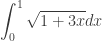
Usually, you can start by considering a = 0 , which means that the \displaystyle \frac{b-a}{n}\cdot k becomes the “x.”. Then rewriting the radicand as \displaystyle 1+3\frac{1}{n}k=1+3\left( a+\frac{1}{n}\cdot k \right), it appears the function is \sqrt{1+3x} and the limit is \displaystyle \int_{0}^{1}{\sqrt{1+3x}}dx=\frac{14}{9}.

The answer choices are

(A)  \displaystyle \int_{0}^{1}{\sqrt{1+3x}}dx        (B)    \displaystyle \int_{0}^{3}{\sqrt{1+x}}dx      (C)    \displaystyle \int_{1}^{4}{\sqrt{x}}dx     (D)   \displaystyle \tfrac{1}{3}\int_{0}^{3}{\sqrt{x}}dx

The correct choice is (A), but notice that choices B, C, and D can be eliminated as soon as we determine that b = a + 1. That is not always the case.

Let’s consider another example:

Example 2: \displaystyle \underset{n\to \infty }{\mathop{\lim }}\,\sum\limits_{k=1}^{n}{\left( {{\left( 2+\frac{3}{n}k \right)}^{2}}\left( \frac{3}{n} \right) \right)}=

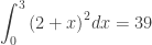
As before consider \displaystyle \frac{b-a}{n}=\frac{3}{n}, which implies that b = a + 3. With a = 0,  the function appears to be {{\left( 2+x \right)}^{2}} on the interval [0, 3], so the limit is \displaystyle \int_{0}^{3}{{{\left( 2+x \right)}^{2}}}dx=39
BUT

What if we take a = 2? If so, the limit is \displaystyle \int_{2}^{5}{{{x}^{2}}dx}=39.

And now one of the “problems” with this kind of question appears: the answer written as a definite integral is not unique!

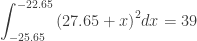
Not only are there two answers, but there are many more possible answers. These two answers are horizontal translations of each other, and many other translations are possible, such as \displaystyle \int_{-25.65}^{-22.65}{{{\left( 27.65+x \right)}^{2}}dx}=39.

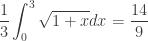
The same thing can occur in other ways. Returning to example 1,and using something like a u-substitution, we can rewrite the original limit as \displaystyle \frac{1}{3}\cdot \underset{n\to \infty }{\mathop{\lim }}\,\sum\limits_{k=1}^{n}{\left( \sqrt{1+\frac{3k}{n}}\cdot \frac{3}{n} \right)}.

Now b = a + 3 and the limit could be either \displaystyle \frac{1}{3}\int_{0}^{3}{\sqrt{1+x}}dx=\frac{14}{9} or \displaystyle \frac{1}{3}\int_{1}^{4}{\sqrt{x}}dx=\frac{14}{9}, among others.

My opinions about this kind of question.

The real problem with the answer choices to Example 1 is that they force the student to do the question in a way that gets one of the answers. It is perfectly reasonable for the student to approach the problem a different way, and get a different correct answer that is not among the choices. This is not good.

The problem could be fixed by giving the answer choices as numbers. These are the numerical values of the 4 choices:(A) 14/9   (B) 14/3   (C)  14/3   (D)    2\sqrt{3}/3. As you can see that presents another problem. Distractors (wrong answers) are made by making predictable calculus mistakes. Apparently, two predictable mistakes give the same numerical answer; therefore, one of them must go.

A related problem is this: The limit of a Riemann sum is a number; a definite integral is a number. Therefore, any definite integral, even one totally unrelated to the Riemann sum, which has the correct numerical value, is a correct answer.

I’m not sure if this type of question has any practical or real-world use. Certainly, setting up a Riemann sum is important and necessary to solve a variety of problems. After all, behind every definite integral there is a Riemann sum. But starting with a Riemann sum and finding the function and interval does not seem to me to be of practical use.

The CED references this question to MPAC 1: Reasoning with definitions and theorems, and to MPAC 5: Building notational fluency. They are appropriate,and the questions do make students unpack the notation.

My opinions notwithstanding, it appears that future exams will include questions like these.


These questions are easy enough to make up. You will probably have your students write Riemann sums with a small value of n when you are teaching Riemann sums leading up to the Fundamental Theorem of Calculus.  You can make up problems like these by stopping after you get to the limit, giving your students just the limit, and having them work backwards to identify the function(s) and interval(s). You could also give them an integral and ask for the associated Riemann sum. Question writers call questions like these reversal questions since the work is done in reverse of the usual way.


Here is the question from 1997, for you to try. The answer is below.

riemann-reversal


Answer B. Hint n = 50


Revised 5-5-2022


Graphing Integrals

The sixth in the Graphing Calculator / Technology series

The topic of integration is coming up soon. Here are some notes and ideas about the integration operation on graphing calculators. The entries are the same or very similar for all calculator brands.

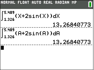
The basic problem of evaluating a definite integral on a graphing calculator is done without finding an antiderivative; that is, the calculator uses a numerical algorithm to produce the result. The calculator provides a template,integral-templateand you fill in the 4 squares so that the expression looks exactly like what you write by hand. Then the calculator computes the result. (Older models require a one-line input requiring, in order, the integrand, the independent variable, the lower limit of integration and the upper limit in that order, separated by commas.) The first interesting thing is that the variable in the integrand does to have to be x. As the first figure illustrates using x or a or any other letter gives the same result.

integral-0

This is because the variable of integration is just a place holder. Sometimes called a “dummy variable”, this letter can be anything at all, including x. On the home or calculation screen you might as well always use x, so the entry will look like what you have on your paper. As we will see, when graphing it may be less confusing to use a different letter.

The antiderivative, F, of any function, f, can be written as a function defined by an integral where there is a point on the antiderivative of f , which is with F ’ = f. The point (aF(a)) is the initial condition. (In the following we will use F(a) = 0 as the initial condition – the graph will contain the origin. As a further investigation, try changing the lower limit to different numbers and see how that changes the graph.)

The integration operation can be used to graph the antiderivative of a function without finding the antiderivative. You may graph the antiderivative when teaching antiderivatives. Have students look at the graph of the antiderivative and guess what that function is.

When graphing use x as the upper limit of integration and a different letter for the variable in the rest of the template. The calculator will use different values of x to calculate the points to be graphed.

The set-up shown in the next figure shows how to enter a function defined by an integral (blue line) and the same function obtained by antidifferentiating (red squares). As you can see the results are the same.

integral-1

In this way, you can explore the functions and their indefinite integrals by graphing.

The Fundamental Theorem of Calculus

Another use of using the graph of an integral is to investigate both parts of the Fundamental Theorem of Calculus (FTC). Roughly speaking, the FTC says that the integral of a derivative of a function is that function, and the derivative of an integral is the integrand.

In the figure below, the same function is entered both ways; the graphs are the same. (Note the x’s in the second line must be x in all four places.)

integral-2

.

Good Question 10 – The Cone Problem

Today’s good question is an optimization problem, but its real point is choosing how to do the computation. As such it relates to MPAC 3a and 3b: “Students can  … select appropriate mathematical strategies [and] sequence algebraic/computational processes logically.” The algebra required to solve this questions can be quite daunting, unless you get clever. Here’s the question.

A sector of arc length x is removed from a circle of radius 10 cm. The remaining part of the circle is formed into a cone of radius r and height h,

  1. Find the value of x so that the cone has the maximum possible volume.
  2. The sector that was removed is also formed into a cone. Find the value of x that makes this cone have it maximum possible volume. (Hint: This is an easy problem.)
  3. In the context of the problem, the expression for the volume of the cone in part a. has a domain of 0\le x\le 20\pi . Why? Ignore the physical situation and determine the domain of the expression for the volume from a. Graph the function. Discuss.

Solutions:

Part a: As usual, we start by assigning some variables.

cone-1

Let r be the radius of the base of the cone and let h be its height. The circumference of the cone is 2\pi r=20\pi -x, so r=10-\frac{x}{2\pi } and h=\sqrt{{{10}^{2}}-{{r}^{2}}}. The volume of the cone is

\displaystyle V=\frac{\pi }{3}{{r}^{2}}h=\frac{\pi }{3}{{r}^{2}}\sqrt{{{10}^{2}}-{{r}^{2}}}=\frac{\pi }{3}{{\left( 10-\frac{x}{2\pi } \right)}^{2}}\sqrt{{{10}^{2}}-{{\left( 10-\frac{x}{2\pi } \right)}^{2}}}

To find the maximum, the next step is to differentiate the volume. The expression on the right above looks way complicated and its derivative will be even worse. Simplifying it is also a lot of trouble, and, in fact, does not make things easier.* Here’s where we can be clever and avoid a lot of algebra. Let’s just work from \displaystyle V=\frac{\pi }{3}{{r}^{2}}\sqrt{{{10}^{2}}-{{r}^{2}}}

To find the maximum differentiate the volume with respect to x using the chain rule.

\displaystyle \frac{dV}{dx}=\frac{dV}{dr}\cdot \frac{dr}{dx}=\frac{\pi }{3}\left( {{r}^{2}}\frac{-2r}{2\sqrt{{{10}^{2}}-{{r}^{2}}}}+2r\sqrt{{{10}^{2}}-{{r}^{2}}} \right)\left( -\frac{1}{2\pi } \right)

Setting this equal to zero and simplifying (multiply by -6\sqrt{{{10}^{2}}-{{r}^{2}}}) gives

-{{r}^{3}}+2r\left( 100-{{r}^{2}} \right)=200r-3{{r}^{3}}=0

\displaystyle r=0,r=\sqrt{\frac{200}{3}}=\frac{10\sqrt{6}}{3}

The minimum is obviously r = 0, so the maximum occurs when  \displaystyle r=10-\frac{x}{2\pi }=\frac{10\sqrt{6}}{3}. Then, solving for x gives

\displaystyle x=2\pi \left( 10-\frac{10\sqrt{6}}{3} \right)\approx 11.52986

Aside: We often see questions saying, if y = f(u) and ug(x), find dy/dx. Here we have put that idea to practical use to save doing a longer computation.

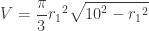
Part b: The arc of the piece cut out is the circumference, x, of a cone with a radius of \displaystyle {{r}_{1}}=\frac{x}{2\pi } and a height of \displaystyle {{h}_{1}}=\sqrt{{{10}^{2}}-{{r}_{1}}^{2}}. Its volume is

\displaystyle V=\frac{\pi }{3}{{r}_{1}}^{2}\sqrt{{{10}^{2}}-{{r}_{1}}^{2}}

This is the same as the expression we used in part a. and can be handled the same way, except that here \displaystyle \frac{d{{r}_{1}}}{dx}=+\frac{1}{2\pi }. The computation and result will be the same. The result will be the same. The maximum occurs at

\displaystyle x=2\pi \left( 10-\frac{10\sqrt{6}}{3} \right)\approx 11.52986

This should not be a surprise.  The piece cut out and the piece that remains are otherwise indistinguishable, so the maximum volume should be the same for both.

Part c: From part a we have \displaystyle V=\frac{\pi }{3}{{r}^{2}}\sqrt{{{10}^{2}}-{{r}^{2}}}=\frac{\pi }{3}{{\left( 10-\frac{x}{2\pi } \right)}^{2}}\sqrt{{{10}^{2}}-{{\left( 10-\frac{x}{2\pi } \right)}^{2}}}. To graph there is no need to simplify the expression in x:
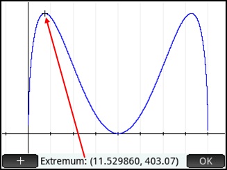
Tthe x scale marks are at multiples of $latex 5\pi $

The x-scale marks are at multiples of 5\pi

The domain is determined by the expression under the radical so

-10\le r\le 10

-10\le 10-\frac{x}{2\pi }\le 10

0\le x\le 40\pi

This is the “natural domain” of the function without regard to the physical situation given in the original problem. I cannot think of a reason for the difference.

________________

*Fully simplified in terms of x the volume is \displaystyle V=\frac{1}{24{{\pi }^{2}}}{{\left( 20\pi -x \right)}^{2}}\sqrt{40\pi x-{{x}^{2}}}. This isn’t really easier to differentiate and solve.

.

From One Side or the Other.

Recently, a reader wrote and suggested my post on continuity would be improved if I discussed one-sided continuity. This, along with one-sided differentiability, is today’s topic.

The definition of continuity requires that for a function to be continuous at a value x = a in its domain \underset{x\to a}{\mathop{\lim }}\,f\left( x \right)=f\left( a \right) and that both values are finite. That is, the limit as you approach the point in question be equal to the value at that point. This limit is a two-sided limit meaning that the limit is the same as x approaches a from both sides. That definition is extended to open intervals, by requiring that for a function to be continuous on an open interval, that it is continuous at every point of the interval

How do you check every point? One way is to prove the limit in the definition in general for any point in the open interval. Another is to develop a list of theorems that allow you to do this. For example, f(x) = x can be shown to be continuous at every number. Then sums, differences, and products, of this function allows you to extend the property to polynomials and then other functions.

But what about a function that has a domain that is not the entire number line? Something like f\left( x \right)=\sqrt{4-{{x}^{2}}},-2\le x\le 2. Here, f\left( -2 \right)=f\left( 2 \right)=0; the function is defined at the endpoints. A look at the graph shows a semi-circle that appears to contain the endpoints (–2, 0) and (2, 0). The function is continuous on the open interval (–2, 2) but cannot be continuous under the regular definition since the limit at the endpoints does not exist. The limit does not exist because the limit from the left at the left-endpoint, and the limit from the right at the right endpoint do not exist. What to do?

continuity

What is done is to require only that the one-sides limits from inside the domain exist. Here they do:\underset{x\to -2+}{\mathop{\lim }}\,f\left( x \right)=0  and the \underset{x\to 2-}{\mathop{\lim }}\,f\left( x \right)=0 and since the limits equal the values we say the function is continuous on the closed interval [–2, 2]. In general, when you say a function is continuous on a closed interval, you mean that the one-sided limits from inside the interval exist and equal the endpoint values.

You can determine that the limits exist by finding them as in the example above. Another way is to realize that if a < b < c < d and the function is continuous on the open (or closed) (a, d) then it is continuous on the closed interval [b c].

Why bother?

The reason we take this trouble is because for some reason the proof of the theorem under consideration requires that the endpoint value not only exist but hooks up with the function to make it continuous. Thus, the continuity on a closed interval is included in the hypotheses of theorem where this property is required. For example, the Intermediate Value Theorem would not work on a function that had no endpoints for f\left( c \right) to be between. Also, the Mean Value Theorem requires you to find the slope between the endpoints, so the endpoint needs to be not only defined, but attached to the rest of the function.

One-sided differentiability

The definition of the derivative at a point also requires a two-sided limit to exist at the point. Most of the early theorems in calculus require only that the function be differentiable on an open interval.

Is it possible to define differentiability at the endpoint of an interval? Yes. It’s done in the same way by using a one-sided limit. If x = a is the left endpoint of an interval, then the derivative from the right at that point is defined as

\displaystyle {f}'\left( a \right)=\underset{h\to 0+}{\mathop{\lim }}\,\frac{f\left( a+h \right)-f\left( a \right)}{h}.

By letting h approach 0 only from the right, you never consider values outside the interval. (At the right endpoint a similar definition is used with h\to 0-).

So why don’t we ever see one-sided derivatives? Because the theorems do not need them to prove their result. Hypotheses of theorems should be the minimum requirements needed, so if there is no need for the function to be differentiable at an endpoint, this is not listed in the hypotheses. This makes the hypothesis less restrictive and, therefore, covers more situations.

One theorem, beyond what is usually covered in beginning calculus, where endpoint differentiability is needed is Darboux’s Theorem. Darboux’s Theorem is sometime called the Intermediate Value Theorem for derivatives. It says that the derivative takes on all values between the derivatives at the endpoints, and thus needs the one-sided derivatives at the endpoints to exist. Interestingly, Darboux’s Theorem does not require the function to be continuous on the open interval between the endpoints.

.